Page 107 - Geometric Modeling and Algebraic Geometry

6 Classification of Surfaces 105
⎛ ⎞
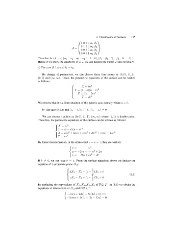
⎜ 1000 α 1 β 1 ⎟
A = ⎜ 0100 α 2 β 2 ⎟ .
⎠
⎝ 0010 α 3 β 3
0001 α 4 β 4
Therefore kerA =< (α 1 : α 2 : α 3 : α 4 : −1:0), (β 1 : β 2 : β 3 : β 4 :0: −1) >.
Hence if we know the equations of Π A , we can deduce the matrix A and reversely.
a) The case (5.1.a) and t 1 = t 2 :

By change of parameters, we can choose these four points as (0, 0), (1, 1),
(0,b) and (∞, ∞). Hence, the parametric equations of the surface can be written
as follows:
⎧
X = tu 2
⎪
⎪
⎨
Y =(t − s)(u − v) 2
Z = t(u − bv) 2
⎪
⎪
T = sv 2
⎩
We observe that it is a limit situation of the generic case, namely where a =0.
b) The case (5.1.b) and (t 1 − t 2 )(t 2 − t 3 )(t 1 − t 3 ) =0:
We can choose 4 points as (0, 0), (1, 1), (∞, ∞) where (1, 1) is double point.
Therefore, the parametric equations of the surface can be written as follows:
⎧
⎪ X = tu 2
⎪
⎨
Y =(t − s)(u − v) 2
⎪ Z = atu + btuv + csu + dtv + esuv + fsv 2
2
2
2
⎪
T = sv 2
⎩
By linear transformation, in the affine chart s = v =1, they are written:
⎧
⎨ x = tu 2
y = −2tu + t − u +2u
2
⎩
z = btu + cu + dt
2
If b =0, we can take b =1. From the surface equations above we deduce the
equation of 3-projective plane Π A :
⎧
1
⎪
⎨ dX 2 − X 3 +(d + )X 5 =0
2 (6.6)
1
⎩ cX 2 − X 4 +(c − )X 5 =0
⎪
2
∗
By replacing the expressions of X 2 ,X 3 ,X 4 ,X 5 of F(2, 2) in (6.6) we obtain the
equations of intersection of Π A and F(2, 2) :
∗

−su(u +2dv)+ tu(2d +1) = 0
−2csuv + tv(v +(2c − 1)u)=0