Page 88 - Geometric Modeling and Algebraic Geometry

86 R. Krasauskas and S. Zube
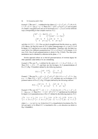
Example 5. The case E ++ is defined by the ellipse c(t)=(1+t ,a(1−t ), 2bt, 0, 0),
2
2
a = p +q , b =2pq, p>q > 0. Then D(t)=(p t +q )(q t +p ) has two pairs
2
2 2
2
2
2 2
2
¯
of complex conjugated roots and can be factorized D(t)= f(t)f(t) in four different
ways corresponding to four complex matrices X(t)

b(t − 1) − 2iat 0 1 0
2
0 1 , 0 b(t − 1) + 2iat ,
2

pt − iq 0 , qt − ip 0 ,
0 qt +ip 0 pt +iq
such that det X(t)= f(t). One can check straightforward that the minors q 01 satisfy
(5.8). Hence, the first two cases of X(t) define Gaussian maps n(t, u) (see (5.7)) of
bi-degree (4, 2) and the last two ones are biquadratic. Therefore, only the latter two
cases define two different parametrizations F(t, u) of Env(C) of bi-degree (4, 2)
(see (5.4)). One of such parametrizations is shown in Fig. 5.5(left). The other para-
metrization can be obtained by reflection in the plane x =0.
Similar approach allows us to find all parametrizations of minimal degree for
other quadratic canal surfaces we are considering.
Example 6. The case P ++ is defined by the curve c(t)=(1, 2a, at , 0, 0), a> 0.
2
Then D(t)= a (1 + t ), and there are two bi-degree (4, 2) parametrizations of
2
2
Env(C) (Fig. 5.5(middle)) defined by the following matrices:

a(t − i) 0 1 0
X(t)= , .
0 1 0 a(t +i)
Example 7. The case H ++ : c(t)=(1−t ,a(1+t ), 2bt, 0, 0), a = p −q , b =2pq,
2
2
2
2
p, q > 0. Then D(t)=(p t + q )(q t + p ), and there are two bi-degree (4, 2)
2
2
2 2
2 2
parametrizations of Env(C) (Fig. 5.5(right)) defined by the following matrices:

pt +iq 0 qt − ip 0
X(t)= , .
0 qt +ip 0 pt − iq
(++) 2 2 2 2
Example 8. The case H : c(t)=(1 − t , 0, 0, 2at, b(1 + t )), a = p + q ,
+−
b =2pq, p, q > 0. Then D(t)=1+2(1−2b /a )t +t , and there are four different
2
4
2
2
bi-degree (4, 2) parametrizations of Env(C) defined by the following matrices X(t):
¯

¯ λt − 1 t + λ i(λt − 1) λt +1 i(λt − 1) λt +1
¯
¯
λt − 1 t + λ
¯
¯
¯
¯
t − λ λt +1 , t − λλt +1 , i(t − λ) t + λ , i(t − λ) t + λ ,
where λ = −(q+ip)/(p+iq). In fact Env(C) is a hyperboloid of revolution (Fig. 5.6,
left and right), or its offsets if C is translated in the x 4 -axis direction (as shown in
Fig. 5.6(middle)).