Page 295 - Glucose Monitoring Devices

302 CHAPTER 15 Automated closed-loop insulin delivery

T
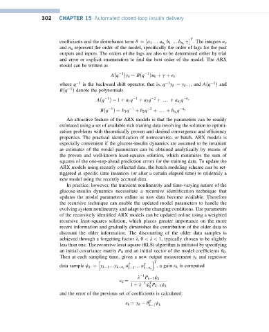
coefficients and the disturbance term q ¼ a 1 . a n y b 1 . b n u g . The integers n y
and n u represent the order of the model, specifically the order of lags for the past
outputs and inputs. The orders of the lags are also to be determined either by trial
and error or explicit enumeration to find the best order of the model. The ARX
model can be written as
1 1
A q y k ¼ B q u k þ g þ ε k
1
1
1
where q is the backward shift operator, that is, q y k ¼ y k 1 , and A q and
1
B q denote the polynomials
1 1 2
A q ¼ 1 þ a 1 q þ a 2 q þ . þ a n y q n y
1 1 2
B q ¼ b 1 q þ b 2 q þ . þ b n y q n y
An attractive feature of the ARX models is that the parameters can be readily
estimated using a set of available rich training data involving the solution to optimi-
zation problems with theoretically proven and desired convergence and efficiency
properties. The practical identification of nonrecursive, or batch, ARX models is
especially convenient if the glucose-insulin dynamics are assumed to be invariant
as estimates of the model parameters can be obtained analytically by means of
the proven and well-known least-squares solution, which minimizes the sum of
squares of the one-step-ahead prediction errors for the training data. To update the
ARX models using recently collected data, the batch modeling scheme can be ret-
riggered at specific time instances (or after a certain elapsed time) to reidentify a
new model using the recently accrued data.
In practice, however, the transient nonlinearity and time-varying nature of the
glucose-insulin dynamics necessitate a recursive identification technique that
updates the model parameters online as new data become available. Therefore
the recursive technique can enable the updated model parameters to handle the
evolving system nonlinearity and adapt to the changing conditions. The parameters
of the recursively identified ARX models can be updated online using a weighted
recursive least-squares solution, which places greater importance on the more
recent information and gradually diminishes the contribution of the older data to
discount the older information. The discounting of the older data samples is
achieved through a forgetting factor l,0 < l < 1, typically chosen to be slightly
less than one. The recursive least square (RLS) algorithm is initiated by specifying
an initial covariance matrix P 0 and an initial vector of the model coefficients q 0 .
Then at each sampling time, given a new output measurement y k and regressor
h i T
u T . u T ,again k k is computed
k
data sample j ¼ y k 1 .y k n y k 1 k n u
1
l P k 1 j k
1 T
k k ¼
k
1 þ l j P k 1 j k
and the error of the previous set of coefficients is calculated:
T
j
e k ¼ y k q k 1 k