Page 534 - Handbook Of Integral Equations

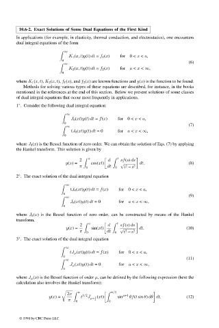
10.6-2. Exact Solutions of Some Dual Equations of the First Kind

In applications (for example, in elasticity, thermal conduction, and electrostatics), one encounters
dual integral equations of the form

∞
K 1 (x, t)y(t) dt = f 1 (x) for 0 < x < a,
0
∞
(6)
K 2 (x, t)y(t) dt = f 2 (x) for a < x < ∞,
0
where K 1 (x, t), K 2 (x, t), f 1 (x), and f 2 (x) are known functions and y(x) is the function to be found.
Methods for solving various types of these equations are described, for instance, in the books
mentioned in the references at the end of this section. Below we present solutions of some classes
of dual integral equations that occur most frequently in applications.
1 . Consider the following dual integral equation:
◦
∞

J 0 (xt)y(t) dt = f(x) for 0 < x < a,
0
∞
(7)
tJ 0 (xt)y(t) dt =0 for a < x < ∞,
0
where J 0 (x) is the Bessel function of zero order. We can obtain the solution of Eqs. (7) by applying
the Hankel transform. This solution is given by

a t
2 d sf(s) ds
y(x)= cos(xt) √ dt. (8)
π 0 dt 0 t – s 2
2
2 . The exact solution of the dual integral equation
◦

∞
tJ 0 (xt)y(t) dt = f(x) for 0 < x < a,
0
(9)
∞
J 0 (xt)y(t) dt =0 for a < x < ∞,
0
where J 0 (x) is the Bessel function of zero order, can be constructed by means of the Hankel
transform,
a t
2 d sf(s) ds
y(x)= sin(xt) √ dt. (10)
π 0 dt 0 t – s 2
2
3 . The exact solution of the dual integral equation
◦

∞
tJ µ (xt)y(t) dt = f(x) for 0 < x < a,
0
(11)
∞
J µ (xt)y(t) dt =0 for a < x < ∞,
0
where J µ (x) is the Bessel function of order µ, can be defined by the following expression (here the
calculation also involves the Hankel transform):
a π/2
2x 3/2 µ+1
y(x)= t J µ+ 1 (xt) sin θf(t sin θ) dθ dt. (12)
π 0 2 0

© 1998 by CRC Press LLC

© 1998 by CRC Press LLC
Page 516