
Page 510 - Handbook of Biomechatronics
P. 510
504 Ahmet Fatih Tabak
asymmetries (Corkidi et al., 2008; Frymier et al., 1995). This type of rigid-
body motion invokes the following combined effects of Basset history inte-
gral and added mass (Wang and Ardekani, 2012; Landau and Lifshitz, 2005),
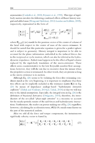
respectively, represented in the form of:
t
2 3
ð
2 p ffiffiffiffiffiffiffiffi ∂U tðÞ dT 2 3 ∂U tðÞ
F t tðÞ 6 6R πμρ p ffiffiffiffiffiffiffiffiffiffiffi πR ρ 7
¼ 6 ∂t t T 3 ∂t 7 (26)
T t tðÞ 4 ∞ 5
head t ðÞ F t tðÞ
p
where P head (t) (m) stands for the position vector of the center of volume of
the head with respect to the center of mass of the micro-swimmer. It
should be noted that this particular equation is given for a perfect sphere
and is subject to geometry. History integral is important to be able to
account for the phase information embedded in the induced forces due
to the reciprocal or cyclic motion, which can also be referred as the hydro-
dynamic impedance. Added mass happens to be the effect of liquid volume
replaced by the rigid-body translation of the micro-swimmer. These
effects seem counterintuitive to the low Reynolds number flow assump-
tions; however, they will die out due to excessive shear the instant when
the propulsive action is terminated. In other words, they are present as long
as the micro-swimmer is in motion.
Although Eq. (26) seems to be violating the force-free swimming con-
dition stated at the very beginning, it is important to emphasize that these
two effects can be implicitly included in the resistance matrix K(t) in Eq.
(20) by means of impedance analogy-based “hydrodynamic interaction
coefficients”(Tabak and Yesilyurt, 2014a,b; Tabak, 2018) so that we will stay
true to the initial assumptions. Especially, the integral term in Eq. (26) is the
definition of fractional derivative (Ortigueira, 2011); therefore, the intro-
duction of the so-called “phase-angle correction” is a necessity to account
for the steady-periodic nature of the said forces and hydrodynamic interac-
tions. Furthermore, the reader can pursue making use of Eq. (26) regardless;
however, calculating the acceleration term, ∂U(t)/∂t, entails some finesse on
the part of the numerical analysis.
After we add all the force and torque components, the instantaneous
rigid-body velocity vector is found by
U tðÞ 1 F p + F c + F f + F m + F e + F g + F t
t
¼ K ðÞ (27)
Ω tðÞ T p + T c + T f + T m + T e + T g + T t