Page 151 - Handbook of Civil Engineering Calculations, Second Edition

1.134 STRUCTURAL STEEL ENGINEERING AND DESIGN

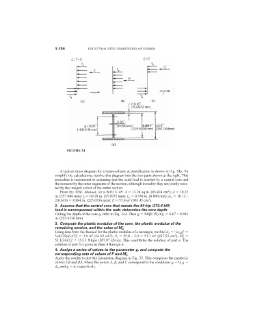
FIGURE 34

A typical stress diagram for a beam-column at plastification is shown in Fig. 34a. To
simplify the calculations, resolve this diagram into the two parts shown at the right. This
procedure is tantamount to assuming that the axial load is resisted by a central core and
the moment by the outer segments of the section, although in reality they are jointly resis-
ted by the integral action of the entire section.
2
From the AISC Manual, for a W10 45: A 13.24 sq.in. (85.424 cm ); d 10.12
in. (257.048 mm); t f 0.618 in. (15.6972 mm); t w 0.350 in. (8.890 mm); d w 10.12 –
3
3
2(0.618) 8.884 in. (225.6536 mm); Z 55.0 in (901.45 cm ).
2. Assume that the central core that resists the 84-kip (373.6-kN)
load is encompassed within the web; determine the core depth
Calling the depth of the core g, refer to Fig. 34d. Then g 84/[0.35(36)] 6.67 < 8.884
in. (225.6536 mm).
3. Compute the plastic modulus of the core, the plastic modulus of the
remaining section, and the value of M p
2
Using data from the Manual for the plastic modulus of a rectangle, we find Z c /4 t w g
1
2
3
3
3
3
1 /4(0.35)(6.67) 3.9 in (63.92 cm ); Z r 55.0 – 3.9 51.1 in (837.53 cm ); M
p
51.1(36)/12 153.3 ft·kips (207.87 kN·m). This constitutes the solution of part a. The
solution of part b is given in steps 4 through 6.
4. Assign a series of values to the parameter g, and compute the
corresponding sets of values of P and M p
Apply the results to plot the interaction diagram in Fig. 35. This comprises the parabolic
curves CB and BA, where the points A, B, and C correspond to the conditions g 0, g
d w , and g d, respectively.