Page 93 - Handbook of Deep Learning in Biomedical Engineering Techniques and Applications

Chapter 3 Application, algorithm, tools directly related to deep learning 81

As shown in Fig. 3.16, the hidden layers are well trained by an
unsupervised algorithm and then fine-tuned by a supervised algo-
rithm. Stacked autoencoder mainly focused on three steps. Train
autoencoder by using input data, and acquire all the learned data.
The learned data from the previous layer is fed back as an input
for the next layer, and this continues until the training is fully
completed. Once all the hidden layers are trained, then use the
backpropagation algorithm to minimize the cost function.
Weights are updated with the training data set to achieve fine-
tuning [19].

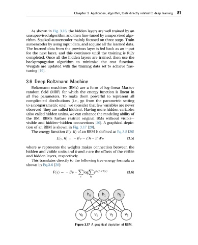
3.6 Deep Boltzmann Machine
Boltzmann machines (BMs) are a form of log-linear Markov
random field (MRF) for which the energy function is linear in
all free parameters. To make them powerful to represent all
complicated distributions (i.e., go from the parametric setting
to a nonparametric one), we consider that few variables are never
observed (they are called hidden). Having more hidden variables
(also called hidden units), we can enhance the modeling ability of
the BM. RBMs further restrict original BMs without visiblee
visible and hiddenehidden connections [20]. A graphical depic-
tion of an RBM is shown in Fig. 3.17 [20].
The energy function Eðy; hÞ of an RBM is defined as Eq.3.5 [20]
Eðy; hÞ¼ b y c h h Wy (3.5)
0
0
0
where w represents the weights makes connection between the
hidden and visible units and b and c are the offsets of the visible
and hidden layers, respectively.
This translates directly to the following free energy formula as
shown in Eq.3.6 [20]:

X X
0 e h i ðc i þW i yÞ
FðyÞ¼ b y log (3.6)
i h i

Figure 3.17 A graphical depiction of RBM.