Page 184 - Hardware Implementation of Finite-Field Arithmetic

166 Cha pte r Se v e n

where poly_vector and poly2_vector are bit vectors from 0 to m – 1, and
0 to 2m – 2, respectively. The total gate complexity for the bit-parallel
2
computation of the matrix-vector product given in Eq. (7.3) is m
2
AND gates and (m – 1) XOR gates ([RSDK06], [PL07]). The AND
,
gates operate all in parallel and require a single AND gate delay T AND
⎡
while the XOR gates are organized as a binary tree of depth log j⎤
2 ⎥
⎢
in order to add j operands. The total time complexity is then found by
considering the largest number of terms, which is equal to m for the
computation of d . Therefore, the total delay complexity for the bit-
m − 1
⎤
parallel matrix-vector product is T + ⎡log m T .
⎢
⎥
AND 2 XOR
After the above polynomial multiplication d(x) = a(x)b(x), a
reduction modulo an irreducible polynomial f(x ) must be performed.
In modular reduction c(x) = d(x) mod f(x), the degree 2m – 2 polynomial
d(x) is reduced by the degree m irreducible polynomial f(x), resulting
in a polynomial c(x) with degree deg(c(x)) ≤ m – 1:
c(x) = d(x) mod f(x) = (d x 2m - 2 + . . . + d x + d ) mod f(x)
2m - 2 1 0
= c x m - 1 + . . . + c x + c (7.5)
m − 1 1 0
Reduction modulo f(x) can be viewed as a linear mapping of the
2m – 1 coefficients of d(x) into the m coefficients of c(x). This mapping
can be represented in a matrix notation as follows [Paa94]:
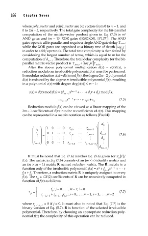
⎛ d 0 ⎞
⎛ c ⎞ ⎛ 10 0 r 00 , r 0, m 2 ⎞ ⎜ ⎟
−
⎜ c 0 ⎟ ⎜ 01 0 r r ⎟ ⎜ d ⎟
⎜ 1 ⎟ = ⎜ 1,,0 , 1 m− 2 ⎟ ⎜ m −1 ⎟ (7.6)
⎜ ⎟ ⎜ ⎟ ⎜ d m ⎟ ⎟
⎜
⎝ c ⎜ m 1⎠ ⎟ ⎜ ⎝ 00 1 r m− , 10 r m− , 1 m− 2⎠ ⎟ ⎠ ⎜ ⎟
−
⎜d ⎟ ⎠
⎝ 2 m −2
It must be noted that Eq. (7.6) matches Eq. (5.6) given for Z [x]/
p
f(x). The matrix in Eq. (7.6) consists of an (m × n) identity matrix and
an (m × m – 1) matrix R named reduction matrix. The R matrix is a
m
function only of the irreducible polynomial f(x) = x + f x m − 1 + . . . +
m − 1
f x + f . Therefore, a reduction matrix R is uniquely assigned to every
1 0
f(x). The r ∈ GF(2) coefficients of R can be recursively computed in
j,i
function of f(x) as follows:
⎧ f ; = 0 ... , m − 1 i ; = 0
⎪
,
j
r = ⎨ j (7.7)
−
−
ji , r + r r ; = , 0 ... , m 1 = , 1 ... , m 2
i ;
j
j
⎩ ⎪ j−1 i , −1 m−1 i , −1 j,0
where r = 0 if j = 0. It must also be noted that Eq. (7.7) is the
j - 1, i - 1
binary version of Eq. (5.7). R is function of the selected irreducible
polynomial. Therefore, by choosing an appropriate reduction poly-
nomial f(x) the complexity of this operation can be reduced.