Page 296 - Hardware Implementation of Finite-Field Arithmetic

276 Cha pte r Ni ne

4
how to perform the squaring over the dual basis in GF(2 ) as given in
Eq. (9.17) is available. Assume also that the function
function dual_mult(Ad,B,F: poly_vector) return poly_
vector;
how to perform the dual basis multiplication as given in Algorithm 9.1
is also available, where the input operand B is represented in the poly-
nomial basis, the input operand Ad and the product are represented in
m
the dual basis, and F is the defining irreducible polynomial for GF(2 ).
Then the following algorithm implements the inversion INV = A − 1
3
4
2
given in Eq. (9.18) over the dual basis {,1 αα α for the field GF(2 )
, }
,
generated by f(x) = x + x + 1.
4
4
4
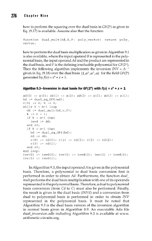
Algorithm 9.3—Inversion in dual basis for GF (2 ) with f (x) = x + x + 1
ad(0) := a(0); ad(1) := a(3); ad(2) := a(2); ad(3) := a(1);
bd := dual_sq_GF4(ad);
c(0) := 1; k := 0;
while k < m-1 loop
dd := dual_mult(bd,c,F);
k := k + 1;
if k = m-1 then
invd := dd;
end if;
if k < m-1 then
bd := dual_sq_GF4(bd);
cd := dd;
c(0) := cd(0); c(1) := cd(3); c(2) := cd(2);
c(3) := cd(1);
end if;
end loop;
inv(0) := invd(0); inv(1) := invd(3); inv(2) := invd(2);
inv(3) := invd(1);

In Algorithm 9.3, the input operand A is given in the polynomial
basis. Therefore, a polynomial to dual basis conversion first is
performed in order to obtain Ad. Furthermore, the function dual_
mult performs the dual basis multiplication with one of its operands
represented in the polynomial basis. Therefore, a dual to polynomial
basis conversion (from Cd to C) must also be performed. Finally,
the result is given in the dual basis (INVd) and a conversion from
dual to polynomial basis is performed in order to obtain INV
represented in the polynomial basis. It must be noted that
Algorithm 9.3 is the dual basis version of the inversion algorithm
in normal basis given in Algorithm 8.9. An executable Ada file
dual_inversion.adb including Algorithm 9.3 is available at www.
arithmetic-circuits.org.