Page 311 - Hardware Implementation of Finite-Field Arithmetic

An Example of Application—Elliptic Curve Cryptography 291

if P = (x , y ), Q = (x , y ), P ≠ Q and P ≠− Q, then P + Q = (x , y )
1 1 2 2 3 3
where
2
x = [(y + y )/(x + x )] + x + x ,
3 1 2 1 2 1 2
(10.20)
y = [(y + y )/(x + x )](x + x ) + y + c
3 1 2 1 2 1 3 1
if P = (x , y ) and P ≠ −P, then P + P = (x , y ) where
1 1 3 3
2
2
2
x = [(x + a)/c] , y = [(x + a)/c](x + x ) + y + c (10.21)
3 1 3 1 1 3 1
The following formal algorithm computes P + Q. The function
adding computes Eq. (10.12), (10.16), or (10.20), while the function
doubling computes Eq. (10.13), (10.17), or (10.21):
Algorithm 10.1—Computation of R = P + Q
if P = point_at_infinity then R := Q;
elsif Q = point_at_infinity then R := P;
elsif P = -Q then R := point_at_infinity;
elsif P = Q then R := doubling(P);
else R := adding(P,Q);
end if;

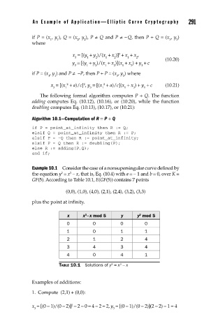
Example 10.1 Consider the case of a nonsupersingular curve defined by
the equation y = x – x, that is, Eq. (10.4) with a =− 1 and b = 0, over K =
3
2
GF(5). According to Table 10.1, E(GF(5)) contains 7 points
(0,0), (1,0), (4,0), (2,1), (2,4), (3,2), (3,3)

plus the point at infinity.

3
2
x x −x mod 5 y y mod 5
0 0 0 0
1 0 1 1
2 1 2 4
3 4 3 4
4 0 4 1
2
3
TABLE 10.1 Solutions of y = x − x

Examples of additions:
1. Compute (2,1) + (0,0):

2
x = [(0 − 1)/(0 − 2)] − 2 − 0 = 4 − 2 = 2, y = [(0 − 1)/(0 − 2)](2 − 2) − 1 = 4
3 3