Page 251 - Innovations in Intelligent Machines

244 J. Gaspar et al.
the scene model and the observed lines as well as possible. This is computa-
tionally more expensive, but more robust to direction errors on the observed
line segments [34].
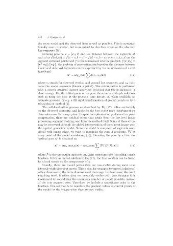
Defining pose as x =[xy θ] and the distance between the segments ab
and cd as d (cd, ab)= f (c − a, b − a)+ f (d − a, b − a) where a, b, c, d are the
segment extremal points and f is the normalised internal product, f(v, v 0 )=
T 0 ⊥ . ⊥. , the problem of pose estimation based on the distance between
. .
v .v
/ v
0
model and observed segments can be expressed by the minimization of a cost
functional:

∗
x =arg min d (s i ,s 0i (x)) (17)
x
i
where s i stands for observed vertical and ground line segments, and s 0i indi-
cates the model segments (known a priori). The minimization is performed
with a generic gradient descent algorithm provided that the initialisation is
close enough. For the initial guess of the pose there are also simple solutions
such as using the pose at the previous time instant or, when available, an
estimate provided by e.g. a 2D rigid transformation of ground points or by a
triangulation method [4].
The self-localisation process as described by Eq. (17), relies exclusively
on the observed segments, and looks for the best robot pose justifying those
observations on the image plane. Despite the optimization performed for pose-
computation, there are residual errors that result from the low-level image
processing, segment tracking, and from the method itself. Some of these errors
may be recovered through the global interpretation of the current image with
the a priori geometric model. Since the model is composed of segments asso-
ciated with image edges, we want to maximize the sum of gradients, ∇I at
every point of the model wire-frame, {P i }. Denoting the pose by x then the
optimal pose x is obtained as:
∗

x =arg max µ(x)=arg max |∇I (P(P i ; x))| (18)
∗
x
x
i
where P is the projection operator and µ(x) represents the (matching) merit
function. Given an initial solution to Eq. (17), the final solution can be found
by a local search on the components of x.
Usually, there are model points that are non-visible during some time
intervals while the robot moves. This is due, for example, to camera (platform)
self-occlusion or to the finite dimensions of the image. In these cases, the merit
matching merit function does not smoothly evolve with pose changes: it is
maximized by considering the maximum number of points possible, instead
of the true segment pose. Therefore, we include a smoothness prior to the
function. One solution is to maintain the gradient values at control points of
the model for the images when they are not visible.