Page 229 - Solutions Manual to accompany Electric Machinery Fundamentals

e_a0 = int erp1(if_values,ea_values,i_f);

% Calculate the resulting speed from Equation (9-13).
n = ( e_a ./ e_a0 ) * n_0;

% Calculate the induced torque corresponding to each
% speed from Equations (8-55) and (8-56).
t_ind = e_a .* i_a ./ (n * 2 * pi / 60);

% Plot the torque-speed curves
figure(1);
plot(t_ind,n ,'b-','LineWidth',2.0);
xlabel('\bf\tau_{ind} (N-m)');
ylabel('\bf\itn_{m} \rm\bf(r/min )');
title ('\bfCumulatively-Compounded DC Motor Torque-Speed
Characteristic');
axis([ 0 125 800 12 00]);
grid on;

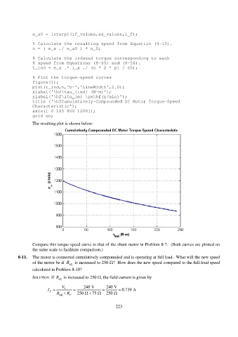
The resulting plot is shown below:

Compare this torque-speed curve to that of the shunt motor in Problem 8-7. (Both curves are plotted on
the same scale to facilitate comparison.)

8-11. The motor is connected cumulatively com pounded and is operating at full load. What will the new speed
of the motor be if R is increased to 250 ? How does the new speed compared to the full-load speed
adj
calculated in Problem 8 -10?

SOLUTION If R is increased to 250 , the field current is given by
adj
V 240 V 240 V
I  F T    0.739 A
R 
adj R F 250   75  250 

223