Page 179 - Materials Chemistry, Second Edition

L1644_C04.fm Page 151 Tuesday, October 21, 2003 3:13 PM

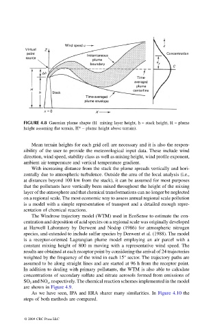
FIGURE 4.8 Gaussian plume shapte (H mixing layer height, h – stack height, H – plume
height assuming flat terrain, H* – plume height above terrain).

Mean terrain heights for each grid cell are necessary and it is also the respon-
sibility of the user to provide the meteorological input data. These include wind
direction, wind speed, stability class as well as mixing height, wind profile exponent,
ambient air temperature and vertical temperature gradient.
With increasing distance from the stack the plume spreads vertically and hori-
zontally due to atmospheric turbulence. Outside the area of the local analysis (i.e.,
at distances beyond 100 km from the stack), it can be assumed for most purposes
that the pollutants have vertically been mixed throughout the height of the mixing
layer of the atmosphere and that chemical transformations can no longer be neglected
on a regional scale. The most economic way to assess annual regional scale pollution
is a model with a simple representation of transport and a detailed enough repre-
sentation of chemical reactions.
The Windrose trajectory model (WTM) used in EcoSense to estimate the con-
centration and deposition of acid species on a regional scale was originally developed
at Harwell Laboratory by Derwent and Nodop (1986) for atmospheric nitrogen
species, and extended to include sulfur species by Derwent et al. (1988). The model
is a receptor-oriented Lagrangian plume model employing an air parcel with a
constant mixing height of 800 m moving with a representative wind speed. The
results are obtained at each receptor point by considering the arrival of 24 trajectories
weighted by the frequency of the wind in each 15° sector. The trajectory paths are
assumed to be along straight lines and are started at 96 h from the receptor point.
In addition to dealing with primary pollutants, the WTM is also able to calculate
concentrations of secondary sulfate and nitrate aerosols formed from emissions of
SO and NO , respectively. The chemical reaction schemes implemented in the model
2
x
are shown in Figure 4.9.
As we have seen, IPA and ERA sharer many similarities. In Figure 4.10 the
steps of both methods are compared.

© 2004 CRC Press LLC