Page 131 - Intelligent Digital Oil And Gas Fields

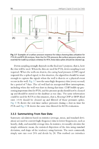
96 Intelligent Digital Oil and Gas Fields

De-noise

(A) PTA (B) RTA Down sampling

Fig. 3.7 Examples of a surface pressure response for 6days showing data utilization for
PTA (A) and RTA (B) analyses. Note that for PTA pressure, the surface pressure spikes are
essential for build-up analysis whereas for RTA, these data spikes should be cleaned up.

Down sampling strongly depends on the final user’s purpose, that is, how
the data will be used. When the data are used for PTA, down sampling is not
required. When the wells are shut in, the casing head pressure (CHP) signal
responds like a spiked signal; in this situation, the algorithm should be smart
enough to capture the signals when the well is shut-in or a physical event
occurs in the well. Fig. 3.7 uses the same high-frequency data (every second)
for a period of 7days. The oil well had six unexpected flow interruptions,
including when the well was shut-in during that time. CHP builds up gen-
erating important data for PTA, and the pressure peaks should not be cleaned
up and should be stored in the database as raw data. The same information
could be used for RTA in this situation, that is, flowing CHP or BHP (fluid
rates >0.0) should be cleaned up and filtered of those pressures spikes.
Fig 3.7A shows the real-time surface pressures during a shut-in time for
PTA and Fig 3.7B shows the same data filtered for RTA evaluation.

3.3.3 Summarizing From Raw Data

Summary calculations based on statistics (average, mean, and standard devi-
ation) are used to convert high-frequency data to lower frequencies, such as
hourly, daily, and monthly average data. In statistics, we usually calculate the
simple arithmetic mean, the statistical dispersion of the data using standard
deviation, and shape of the tendency using kurtosis. The users commonly
simply sum rate over 24h and divide by 24. This method can introduce