Page 47 - Intro Predictive Maintenance

38 An Introduction to Predictive Maintenance

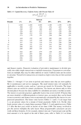
Table 2–5 Capital Recovery, Uniform Series with Present Value $1
(
1
Ê i + i) n ˆ
CP = PÁ ˜
n
( Ë 1 + i) - ¯ 1
Interest
Periods 1% 2% 4% 10% 15% 20%
1 1.010 1.020 1.040 1.100 1.150 1.200
2 .508 .515 .530 .576 .615 .654
3 .340 .347 .360 .402 .438 .475
4 .256 .263 .275 .315 .350 .386
5 .206 .212 .225 .264 .298 .334
6 .173 .179 .191 .230 .264 .301
7 .149 .155 .167 .205 .240 .277
8 .131 .137 .149 .187 .223 .261
9 .117 .122 .135 .174 .210 .248
10 .106 .111 .123 .163 .199 .239
11 .096 .102 .114 .154 .191 .231
12 .089 .095 .107 .147 .184 .225
18 .061 .067 .079 .120 .163 .208
24 .047 .053 .066 .111 .155 .203
36 .0033 .038 .051 .094 .151 .200
48 .026 .032 .045 .092 .150 .200
60 .022 .028 .043 .091 .150 .200

and finance experts. Financial evaluation of preventive maintenance is divided gen-
erally into either single transactions or multiple transactions. If payment or cost reduc-
tions are multiple, they may be either uniform or varied. Uniform series are the easiest
to calculate. Nonuniform transactions are treated as single events that are then summed
together.

Tables 2–1 through 2–5 are done in periods and interest rates that are most applica-
ble to maintenance and service managers. The small interest rates will normally be
applicable to monthly events, such as 1 percent per month for 24 months. The larger
interest rates are useful for annual calculations. The factors are shown only to three
decimal places because the data available for calculation are rarely even that accurate.
The intent is to provide practical, applicable factors that avoid overkill. If factors that
are more detailed, or different periods or interest rates, are needed, they can be found
in most economics and finance texts or automatically calculated by the macros in com-
puterized spreadsheets. The future value factors (Tables 2–1 and 2–3) are larger than
1, as are present values for a stream of future payments (Table 2–4). On the other
hand, present value of a single future payment (Table 2–2) and capital recovery (Table
2–5 after the first year) result in factors of less than 1.000. The money involved to
give the answer multiplies the table factor. Many programmable calculators can also
work out these formulas. If, for example, interest rates are 15 percent per year and the
total amount is to be repaid at the end of three years, refer to Table 2–1 on future