Page 142 - Intro to Tensor Calculus

137

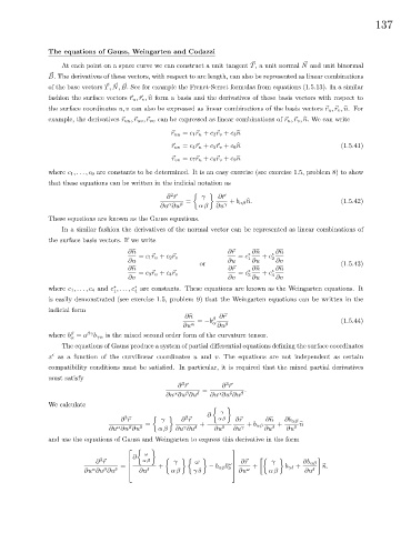
The equations of Gauss, Weingarten and Codazzi
~
~
At each point on a space curve we can construct a unit tangent T, a unit normal N and unit binormal
~
B. The derivatives of these vectors, with respect to arc length, can also be represented as linear combinations
~ ~ ~
of the base vectors T, N, B. See for example the Frenet-Serret formulas from equations (1.5.13). In a similar
fashion the surface vectors ~ u ,~r v , bn form a basis and the derivatives of these basis vectors with respect to
r
the surface coordinates u, v can also be expressed as linear combinations of the basis vectors ~ u ,~r v , bn.For
r
r
example, the derivatives ~ uu ,~r uv ,~r vv can be expressed as linear combinations of ~r u ,~r v , bn. We can write
r
~ uu = c 1~r u + c 2~r v + c 3 bn
~ uv = c 4~r u + c 5~r v + c 6 bn (1.5.41)
r
r
~ vv = c 7~r u + c 8~r v + c 9 bn
where c 1 ,...,c 9 are constants to be determined. It is an easy exercise (see exercise 1.5, problem 8) to show
that these equations can be written in the indicial notation as
2
r
∂ ~r γ ∂~
= + b αβ bn. (1.5.42)
α
∂u ∂u β αβ ∂u γ
These equations are known as the Gauss equations.
In a similar fashion the derivatives of the normal vector can be represented as linear combinations of
the surface basis vectors. If we write
∂bn ∂~ r ∗ ∂bn ∗ ∂bn
= c 1~r u + c 2~r v = c 1 + c 2
∂u ∂u ∂u ∂v
or (1.5.43)
∂bn ∂~ ∗ ∂bn ∗ ∂bn
r
= c 3~r u + c 4~r v = c 3 + c 4
∂v ∂v ∂u ∂v
∗
∗
where c 1 ,...,c 4 and c ,...,c are constants. These equations are known as the Weingarten equations. It
4
1
is easily demonstrated (see exercise 1.5, problem 9) that the Weingarten equations can be written in the
indicial form
∂bn β ∂~
r
= −b α (1.5.44)
∂u α ∂u β
β
where b = a βγ b γα is the mixed second order form of the curvature tensor.
α
The equations of Gauss produce a system of partial differential equations defining the surface coordinates
i
x as a function of the curvilinear coordinates u and v. The equations are not independent as certain
compatibility conditions must be satisfied. In particular, it is required that the mixed partial derivatives
must satisfy
3
3
∂ ~r ∂ ~r
= .
β
α
α
δ
∂u ∂u ∂u δ ∂u ∂u ∂u β
We calculate

γ
∂

2

3
∂ ~r γ ∂ ~r αβ ∂~ r ∂bn ∂b αβ
= + + b αβ + b n
β
α
γ
∂u ∂u ∂u δ αβ ∂u ∂u δ ∂u δ ∂u γ ∂u δ ∂u δ
and use the equations of Gauss and Weingarten to express this derivative in the form
 
ω
∂
3
∂ ~r  αβ γ ω  ∂~r γ ∂b αβ
=  + − b αβ b ω  + b γδ + b n.
∂u ∂u ∂u δ  ∂u δ αβ γδ δ  ∂u ω αβ ∂u δ
β
α