Page 222 - Intro to Tensor Calculus

216

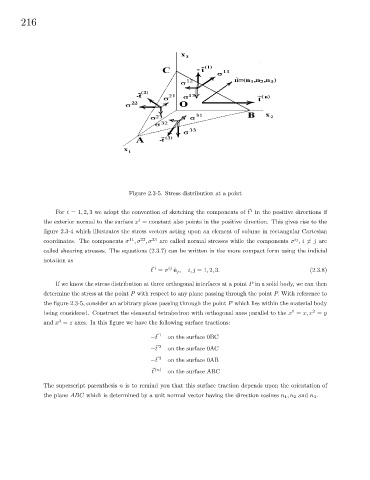
Figure 2.3-5. Stress distribution at a point

i
For i =1, 2, 3 we adopt the convention of sketching the components of ~ t in the positive directions if
i
the exterior normal to the surface x = constant also points in the positive direction. This gives rise to the
figure 2.3-4 which illustrates the stress vectors acting upon an element of volume in rectangular Cartesian
ij
11
22
coordinates. The components σ ,σ ,σ 33 are called normal stresses while the components σ ,i 6= j are
called shearing stresses. The equations (2.3.7) can be written in the more compact form using the indicial
notation as
i
ij
~ t = σ ˆ e j , i, j =1, 2, 3. (2.3.8)
If we know the stress distribution at three orthogonal interfaces at a point P in a solid body, we can then
determine the stress at the point P with respect to any plane passing through the point P. With reference to
the figure 2.3-5, consider an arbitrary plane passing through the point P which lies within the material body
1
2
being considered. Construct the elemental tetrahedron with orthogonal axes parallel to the x = x, x = y
3
and x = z axes. In this figure we have the following surface tractions:
− ~ t 1 on the surface 0BC
− ~ t 2 on the surface 0AC

− ~ t 3 on the surface 0AB
~ t (n) on the surface ABC

The superscript parenthesis n is to remind you that this surface traction depends upon the orientation of
the plane ABC which is determined by a unit normal vector having the direction cosines n 1 ,n 2 and n 3 .