Page 219 - Intro to Tensor Calculus

213

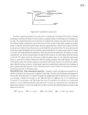
Figure 2.3-2. Typical Stress-strain curve.

Consider a typical stress-strain curve, such as the one illustrated in the figure 2.3-2, which is obtained
by placing a material in the shape of a rod or wire in a machine capable of performing tensile straining at a
low rate. The engineering stress is the tensile force F divided by the original cross sectional area A 0 . Note
that during a tensile straining the cross sectional area A of the sample is continually changing and getting
smaller so that the actual stress will be larger than the engineering stress. Observe in the figure 2.3-2 that
the stress-strain relation remains linear up to a point labeled the proportional limit. For stress-strain points
in this linear region the Hooke’s law holds and the material will return to its original shape when the loading
is removed. For points beyond the proportional limit, but less than the yield point, the material no longer
obeys Hooke’s law. In this nonlinear region the material still returns to its original shape when the loading
is removed. The region beyond the yield point is called the plastic region. At the yield point and beyond,
there is a great deal of material deformation while the loading undergoes only small changes. For points
in this plastic region, the material undergoes a permanent deformation and does not return to its original
shape when the loading is removed. In the plastic region there usually occurs deformation due to slipping of
atomic planes within the material. In this introductory section we will restrict our discussions of material
stress-strain properties to the linear region.
EXAMPLE 2.3-1. (One dimensional elasticity) Consider a circular rod with cross sectional area A
which is subjected to an external force F applied to both ends. The figure 2.3-3 illustrates what happens to
the rod after the tension force F is applied. Consider two neighboring points P and Q on the rod, where P
is at the point x and Q is at the point x +∆x. When the force F is applied to the rod it is stretched and
0
P moves to P and Q moves to Q . We assume that when F is applied to the rod there is a displacement
0
function u = u(x, t) which describes how each point in the rod moves as a function of time t. If we know the
displacement function u = u(x, t) we would then be able to calculate the following distances in terms of the
displacement function

PP = u(x, t), 0P = x + u(x, t), QQ = u(x +∆x, t) 0Q = x +∆x + u(x +∆x, t).
0
0
0
0