Page 214 - Intro to Tensor Calculus

209

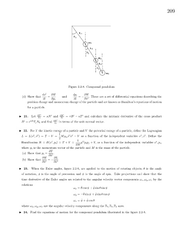
Figure 2.2-8. Compound pendulum

dx i ∂H dp i ∂H
(d) Show that = and = − . These are a set of differential equations describing the
dt ∂p i dt ∂x i
position change and momentum change of the particle and are known as Hamilton’s equations of motion
for a particle.

i
i
i
I 21. Let δT i = κN and δN i = τB − κT and calculate the intrinsic derivative of the cross product
δs δs
i
B = ijk T j N k and find δB i in terms of the unit normal vector.
δs
I 22. For T the kinetic energy of a particle and V the potential energy of a particle, define the Lagrangian
1 i j i i
i
i
L = L(x , ˙x )= T − V = Mg ij ˙x ˙x − V as a function of the independent variables x , ˙x . Define the
2
1 ij i
i
Hamiltonian H = H(x ,p i )= T + V = g p i p j + V, as a function of the independent variables x ,p i ,
2M
where p i is the momentum vector of the particle and M is the mass of the particle.
∂T
(a) Show that p i = .
∂ ˙x i
∂H ∂L
(b) Show that = −
∂x i ∂x i
I 23. When the Euler angles, figure 2.2-6, are applied to the motion of rotating objects, θ is the angle
of nutation, φ is the angle of precession and ψ is the angle of spin. Take projections and show that the
time derivative of the Euler angles are related to the angular velocity vector components ω x ,ω y ,ω z by the
relations
˙
˙
ω x = θ cos ψ + φ sin θ sin ψ
˙
˙
ω y = −θ sin ψ + φ sin θ cos ψ
˙
˙
ω z = ψ + φ cos θ
where ω x ,ω y ,ω z are the angular velocity components along the x 1 , x 2 , x 3 axes.
I 24. Find the equations of motion for the compound pendulum illustrated in the figure 2.2-8.