Page 23 - Intro to Tensor Calculus

19

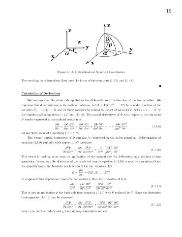
Figure 1.1-5. Cylindrical and Spherical Coordinates

The resulting transformations then have the forms of the equations (1.1.7) and (1.1.8).

Calculation of Derivatives
We now consider the chain rule applied to the differentiation of a function of the bar variables. We
2
1
n
represent this differentiation in the indicial notation. Let Φ = Φ(x , x ,... , x ) be a scalar function of the
i
i
variables x , i =1,... ,N and let these variables be related to the set of variables x , with i =1,... ,N by
the transformation equations (1.1.7) and (1.1.8). The partial derivatives of Φ with respect to the variables
i
x can be expressed in the indicial notation as
∂Φ ∂Φ ∂x j ∂Φ ∂x 1 ∂Φ ∂x 2 ∂Φ ∂x N
= = 1 + 2 + ··· + (1.1.9)
j
∂x i ∂x ∂x i ∂x ∂x i ∂x ∂x i ∂x N ∂x i
for any fixed value of i satisfying 1 ≤ i ≤ N.
The second partial derivatives of Φ can also be expressed in the index notation. Differentiation of
equation (1.1.9) partially with respect to x m produces
2
2 j
∂ Φ ∂Φ ∂ x ∂ ∂Φ ∂x j
= + . (1.1.10)
j
∂x ∂x m ∂x ∂x ∂x m ∂x m ∂x j ∂x i
i
i
This result is nothing more than an application of the general rule for differentiating a product of two
quantities. To evaluate the derivative of the bracketed term in equation (1.1.10) it must be remembered that
the quantity inside the brackets is a function of the bar variables. Let
∂Φ 1 2 N
G = = G(x , x ,..., x )
∂x j
to emphasize this dependence upon the bar variables, then the derivative of G is
2
∂G ∂G ∂x k ∂ Φ ∂x k
= = . (1.1.11)
k
j
k
∂x m ∂x ∂x m ∂x ∂x ∂x m
This is just an application of the basic rule from equation (1.1.9) with Φ replaced by G. Hence the derivative
from equation (1.1.10) can be expressed
2
j
2 j
2
∂ Φ ∂Φ ∂ x ∂ Φ ∂x ∂x k
= + (1.1.12)
i
j
i
i
k
j
∂x ∂x m ∂x ∂x ∂x m ∂x ∂x ∂x ∂x m
where i, m are free indices and j, k are dummy summation indices.