Page 42 - Intro to Tensor Calculus

38

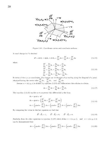
Figure 1.2-1. Coordinate curves and coordinate surfaces.

r
A small change in ~ is denoted
r
∂~ r ∂~ ∂~
r
d~ = dx b e 1 + dy b e 2 + dz b e 3 = du + dv + dw (1.2.15)
r
∂u ∂v ∂w
where
∂~ r ∂x ∂y ∂z
= b e 1 + b e 2 + b e 3
∂u ∂u ∂u ∂u
r
∂~ ∂x ∂y ∂z
= b e 1 + b e 2 + b e 3 (1.2.16)
∂v ∂v ∂v ∂v
r
∂~ ∂x ∂y ∂z
= b e 1 + b e 2 + b e 3 .
∂w ∂w ∂w ∂w
In terms of the u, v, w coordinates, this change can be thought of as moving along the diagonal of a paral-
r
r
∂~ ∂~ ∂~
r
lelepiped having the vector sides du, dv, and dw.
∂u ∂v ∂w
Assume u = u(x, y, z) is defined by equation (1.2.9) and differentiate this relation to obtain
∂u ∂u ∂u
du = dx + dy + dz. (1.2.17)
∂x ∂y ∂z
The equation (1.2.15) enables us to represent this differential in the form:
du = grad u · d~
r

r
r
∂~ ∂~ ∂~
r
du = grad u · du + dv + dw
∂u ∂v ∂w (1.2.18)

∂~ ∂~ r ∂~ r
r
du = grad u · du + gradu · dv + grad u · dw.
∂u ∂v ∂w
By comparing like terms in this last equation we find that
~ 1 ~
~ 1 ~
~ 1 ~
E · E 1 =1, E · E 2 =0, E · E 3 =0. (1.2.19)
Similarly, from the other equations in equation (1.2.9) which define v = v(x, y, z), and w = w(x, y, z)it
can be demonstrated that

r
r
∂~ ∂~ r ∂~
dv = grad v · du + grad v · dv + grad v · dw (1.2.20)
∂u ∂v ∂w