Page 56 -

2.1 Poisson’s Equation in One Dimension
43
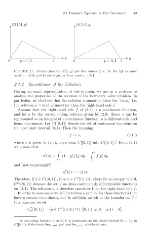
G(3/4,y)
G(1/4,y)

y
y
1
0
1
y =1/4
y =3/4
0
FIGURE 2.1. Green’s function G(x, y) for two values of x. To the left we have
used x =1/4, and to the right we have used x =3/4.
2.1.2 Smoothness of the Solution
Having an exact representation of the solution, we are in a position to
analyze the properties of the solution of the boundary value problem. In
particular, we shall see that the solution is smoother than the “data,” i.e.
the solution u = u(x) is smoother than the right-hand side f.
Assume that the right-hand side f of (2.1) is a continuous function,
and let u be the corresponding solution given by (2.9). Since u can be
represented as an integral of a continuous function, u is differentiable and

hence continuous. Let C (0, 1) denote the set of continuous functions on
the open unit interval (0, 1). Then the mapping
f → u, (2.10)

where u is given by (2.9), maps from C [0, 1] into C [0, 1] . From (2.7)
1
we obtain that
x
1

u (x)= (1 − y)f(y) dy − f(y) dy
0 0
and (not surprisingly!)
u (x)= −f(x).

Therefore, if f ∈ C (0, 1) , then u ∈ C (0, 1) , where for an integer m ≥ 0,
2

C m (0, 1) denotes the set of m-times continuously differentiable functions
on (0, 1). The solution u is therefore smoother than the right-hand side f.
In order to save space we will introduce a symbol for those functions that
have a certain smoothness, and in addition vanish at the boundaries. For
this purpose, we let

C (0, 1) = g ∈ C (0, 1) ∩ C [0, 1] | g(0) = g(1)=0 .
2
2
0
1 A continuous function g on (0, 1) is continuous on the closed interval [0, 1], i.e. in
C [0, 1] , if the limits lim x→0 + g(x) and lim x→1 − g(x) both exist.