Page 414 - Introduction to AI Robotics

11.5 HIMM

III 397

+3
I
-1
II
-1
-1

-1

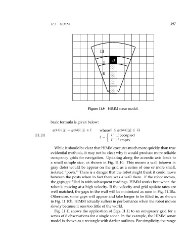
Figure 11.9 HIMM sonar model.

basic formula is given below:
j
g r[i][ i d g r[i][ i d = where 0 g r[i][ i d 15
]
j
]
j
+
I
]
+
(11.11) I if occupied
I =
I if empty
While it should be clear that HIMM executes much more quickly than true
evidential methods, it may not be clear why it would produce more reliable
occupancy grids for navigation. Updating along the acoustic axis leads to
a small sample size, as shown in Fig. 11.10. This means a wall (shown in
gray dots) would be appear on the grid as a series of one or more small,
isolated “posts.” There is a danger that the robot might think it could move
between the posts when in fact there was a wall there. If the robot moves,
the gaps get filled in with subsequent readings. HIMM works best when the
robot is moving at a high velocity. If the velocity and grid update rates are
well matched, the gaps in the wall will be minimized as seen in Fig. 11.10a.
Otherwise, some gaps will appear and take longer to be filled in, as shown
in Fig. 11.10b. HIMM actually suffers in performance when the robot moves
slowly because it sees too little of the world.
Fig. 11.11 shows the application of Eqn. 11.11 to an occupancy grid for a
series of 8 observations for a single sonar. In the example, the HIMM sonar
model is shown as a rectangle with darker outlines. For simplicity, the range