Page 187 - Introduction to Autonomous Mobile Robots

172

a Chapter 4

b

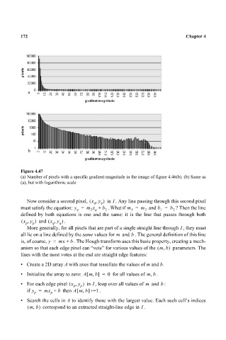
Figure 4.47
(a) Number of pixels with a specific gradient magnitude in the image of figure 4.46(b). (b) Same as
(a), but with logarithmic scale

Now consider a second pixel, x y ) in . Any line passing through this second pixel
,
(
I
q q
must satisfy the equation: y = m x + b . What if m = m and b = b ? Then the line
q 2 q 2 1 2 1 2
defined by both equations is one and the same: it is the line that passes through both
( x y, p ) and x y,( q q ) .
p
I
More generally, for all pixels that are part of a single straight line through , they must
all lie on a line defined by the same values for m and . The general definition of this line
b
is, of course, y = mx + b . The Hough transform uses this basic property, creating a mech-
anism so that each edge pixel can “vote” for various values of the mb,( ) parameters. The
lines with the most votes at the end are straight edge features:
• Create a 2D array A with axes that tessellate the values of m and b.
• Initialize the array to zero: Amb,[ ] = 0 for all values of mb, .
• For each edge pixel x y,( p p ) in , loop over all values of m and : b
I
if y = mx + b then Amb,[ ]+=1 .
p
p
• Search the cells in A to identify those with the largest value. Each such cell’s indices
,
( mb) correspond to an extracted straight-line edge in . I