Page 184 - Introduction to Autonomous Mobile Robots

Perception

a b 169

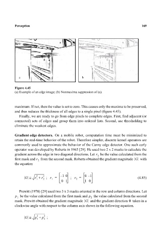
Figure 4.45
(a) Example of an edge image; (b) Nonmaxima suppression of (a).

maximum. If not, then the value is set to zero. This causes only the maxima to be preserved,
and thus reduces the thickness of all edges to a single pixel (figure 4.45).
Finally, we are ready to go from edge pixels to complete edges. First, find adjacent (or
connected) sets of edges and group them into ordered lists. Second, use thresholding to
eliminate the weakest edges.

Gradient edge detectors. On a mobile robot, computation time must be minimized to
retain the real-time behavior of the robot. Therefore simpler, discrete kernel operators are
commonly used to approximate the behavior of the Canny edge detector. One such early
operator was developed by Roberts in 1965 [29]. He used two 2 x 2 masks to calculate the
gradient across the edge in two diagonal directions. Let r be the value calculated from the
1
first mask and r 2 from the second mask. Roberts obtained the gradient magnitude G with
the equation

–
1
G ≅ r + r 2 2 ; r = –0 ; r = 01 (4.85)
2
1
1
2
01 10
Prewitt (1970) [29] used two 3 x 3 masks oriented in the row and column directions. Let
p be the value calculated from the first mask and p the value calculated from the second
1 2
θ
mask. Prewitt obtained the gradient magnitude G and the gradient direction taken in a
clockwise angle with respect to the column axis shown in the following equation.
2
G ≅ p + p 2 ;
1 2