Page 105 - Introduction to Computational Fluid Dynamics

P1: IWV
11:7
May 25, 2005
0 521 85326 5
CB908/Date
0521853265c04
84
JN + 1 2D BOUNDARY LAYERS
∆ y
E Boundary JN
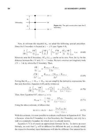
∆ y Figure 4.4. The grid construction near the E
boundary.
JN − 1

Now, to estimate the required ˙ m E , we adopt the following special procedure.
Since the E boundary is located at j = JN (see Figure 4.4),
−1 2

∂ ∂ ∂ ∂ ∂
∂

r
=
+ r JN . (4.68)
∂ ∂y JN ∂y ∂y 2 ∂y ∂y JN
However, near the E boundary, ∂
/∂y| JN can be set to zero. Now, let y be the
distance between the JN and JN − 1 nodes. We next construct an imaginary node
JN + 1at y above the E boundary. Then,

∂ JN+1 − JN−1
= ,
∂y 2 y
JN
2
∂ JN+1 − 2 JN + JN−1
= . (4.69)
∂y 2 y 2
JN
Noting that JN+1 = JN = ∞ , we can simplify the derivative expressions fur-
ther and, therefore, Equation 4.68 can be written as

∂ ∂ r
2r JN
r

2 = . (4.70)
∂ ∂y JN y JN y JN − y JN−1
Thus, from Equation 4.67, since r JN = r E
1 ∂ψ E 2
,E
˙ m E,std
−
. (4.71)
r E ∂x y JN − y JN−1
Using the above estimate, it follows that
2r E
,E x
ψ E (x)
ψ E (x − x) − . (4.72)
y JN − y JN−1
With this estimate, it is now possible to evaluate coefficients in Equation 4.43. This
is because, when the E boundary is a free boundary, the I boundary can only be a
wall or a symmetry boundary for which ψ I (x) is already known.
Equation 4.71 is of course an approximate formula for ˙ m E . To derive an exact
formula, we note that
will be different for different s and, as already noted,
the respective boundary layer thicknesses will also be different. Our interest lies in