Page 110 - Introduction to Computational Fluid Dynamics

P1: IWV
CB908/Date
0 521 85326 5
0521853265c04
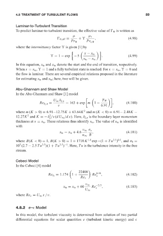
4.8 TREATMENT OF TURBULENT FLOWS
Laminar-to-Turbulent Transition May 25, 2005 11:7 89
To predict laminar-to-turbulent transition, the effective value of
is written as
µ µ t

,eff = + ϒ , (4.98)
Pr Pr t,
where the intermittancy factor ϒ is given [1] by

x − x ts
ϒ = 1 − exp −5 . (4.99)
x te − x ts
In this equation, x ts and x te denote the start and the end of transition, respectively.
When x = x te , ϒ = 1 and a fully turbulent state is reached. For x = x ts , ϒ = 0 and
the flow is laminar. There are several empirical relations proposed in the literature
for estimating x ts and x te ; here, two will be given.

Abu-Ghannam and Shaw Model
In the Abu-Ghannam and Shaw [1] model

U ∞ δ 2,s Tu
Re δ 2 ,s = = 163 + exp m 1 − , (4.100)
ν 6.91
2
where m (K > 0) = 6.91−12.75K + 63.64K and m (K < 0) = 6.91− 2.48K −
2
2
12.27K and K =−δ /ν (dU ∞ /dx). Here, δ 2,s is the boundary layer momentum
2
thickness at x = x ts . These relations thus identify x ts . The value of x te is identified
with
ν ∞ σ o
x te = x ts + 4.6 , (4.101)
u ∞ B
3.5 0.5
where B(K < 0) = 1, B(K > 0) = 1 + 1710 K 1.4 exp −(1 + Tu ) , and σ 0 =
3.5 −1
5
3.5
10 (2.7 − 2.5 Tu )(1 + Tu ) . Here, Tu is the turbulence intensity in the free
stream.
Cebeci Model
In the Cebeci [4] model

22400 0.46
= 1.174 1 + Re , (4.102)
Re δ 2 x
Re x
ν ∞ −2/3
x te = x ts + 60 Re x , (4.103)
U ∞
where Re x = U ∞ x /ν.

4.8.2 e– Model

In this model, the turbulent viscosity is determined from solution of two partial
differential equations for scalar quantities e (turbulent kinetic energy) and