Page 111 - Introduction to Computational Fluid Dynamics

P1: IWV
11:7
May 25, 2005
0 521 85326 5
CB908/Date
0521853265c04
90
3
(turbulent energy dissipation ). Thus, 2D BOUNDARY LAYERS
e 2
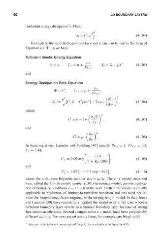
µ t = C µ ρ . (4.104)

Fortunately, the modelled equations for e and can also be cast in the form of
Equation 4.1. Thus, we have
Turbulent Kinetic Energy Equation
µ t
= e,
e = µ + , S e = G − ρ ∗ (4.105)
Pr t,e
and

Energy Dissipation Rate Equation

µ t
= ,
= µ + ,
∗
∗
Pr t, ∗
2
∗ ∂ u 2
∗
S = [C 1 G − C 2 ρ ] + 2νµ t , (4.106)
∗
e ∂y 2
where
√ 2
∂ e
∗
= − 2ν , (4.107)
∂y
and
∂u
2
G = µ t . (4.108)
∂y
In these equations, Launder and Spalding [40] specify Pr t,e = 1, Pr t, = 1.3,
∗
C 1 = 1.44,
−3.4

C µ = 0.09 exp , (4.109)
(1 + Re t /50) 2
and
2
C 2 = 1.92 1 − 0.3exp −Re t , (4.110)
where the turbulence Reynolds number Re t = µ t /µ. The e− model described
here, called the Low Reynolds number (LRE) turbulence model, permits applica-
tion of boundary conditions e = = 0 at the wall. Further, the model is equally
∗
applicable to prediction of laminar-to-turbulent transition and one need not in-
voke the intermittency factor required in the mixing length model. In fact, Jones
and Launder [30] have successfully applied the model even to the case where a
turbulent boundary layer reverts to a laminar boundary layer becuase of strong
free-stream acceleration. Several changes to the e– model have been proposed by
different authors. The more recent among these, for example, are listed in [9].

3 Here ρ is the turbulent counterpart of the µ v term introduced in Equation 4.85.