Page 113 - Introduction to Computational Fluid Dynamics

P1: IWV
0 521 85326 5
May 25, 2005
11:7
0521853265c04
CB908/Date
92
2D BOUNDARY LAYERS
6.Reset y j , r j using the u j just calculated. Also reset ψ b for a free boundary
(b = EorI).
7.Go to step 5 and repeat until convergence of all relevant s is reached.
8.Calculate integral quantities δ 1 , δ 2 , C fx , St x , etc.
u
9.Set x u = x d and = P and return to step 3 to execute a new step.
P
10.Continue untill the domain of interest in the x direction is covered.
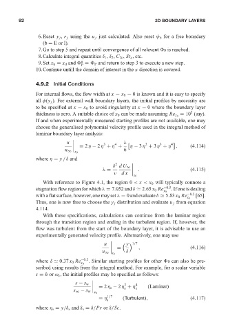
4.9.2 Initial Conditions
For internal flows, the flow width at x = x 0 = 0 is known and it is easy to specify
all φ(y j ). For external wall boundary layers, the initial profiles by necessity are
to be specified at x = x 0 to avoid singularity at x = 0 where the boundary layer
3
= 10 (say).
thickness is zero. A suitable choice of x 0 can be made assuming Re x 0
If and when experimentally measured starting profiles are not available, one may
choose the generalised polynomial velocity profile used in the integral method of
laminar boundary layer analysis:

u 3 4 λ 2 3 4
= 2η − 2η + η + η − 3η + 3η + η , (4.114)
6
u ∞ x 0
where η = y /δ and
2
δ dU ∞
λ = . (4.115)
ν dx
x 0
With reference to Figure 4.1, the region 0 < x < x 0 will typically connote a
stagnation flow region for which λ = 7.052 and δ
2.65 x 0 Re −0.5 . If one is dealing
x 0
with a flat surface, however, one may set λ = 0 and evaluate δ
5.83 x 0 Re −0.5 [65].
x 0
Thus, one is now free to choose the y j distribution and evaluate u j from equation
4.114.
With these specifications, calculations can continue from the laminar region
through the transition region and ending in the turbulent region. If, however, the
flow was turbulent from the start of the boundary layer, it is advisable to use an
experimentally generated velocity profile. Alternatively, one may use
y

1/7
u
= , (4.116)
δ
u ∞ x 0
where δ
0.37 x 0 Re −0.2 . Similar starting profiles for other s can also be pre-
x 0
scribed using results from the integral method. For example, for a scalar variable
s = h or ω k , the initial profiles may be specified as follows:

s − s w 3 4
= 2η s − 2η + η (Laminar)
s s

s ∞ − s w x 0
= η 1/7 (Turbulent), (4.117)
s
where η s = y/δ s and δ s = δ/Pr or δ/Sc.