Page 485 - Introduction to Continuum Mechanics

Non-Newtonian Fluids 469

This is the same relaxation function which we obtained for the spring-dashpot model in
Eq.(8.1.7). In arriving at Eq. (8.1.7), we made use of the initial condition r 0 = G e 0, which was
obtained from considerations of the responses of the elastic element. Here in the present
example, the initial condition is obtained by integrating the differential equation, Eq. (iii), over
an infinitesimal time interval (fromf=Q- tof= 0+). By comparing Eq. (8.1.13) here with Eq.
(8.1.8) of the mechanical model, we see that j is the equivalent of the spring constant G of the
mechanical model. It gives a measure of the elasticity of the linear Maxwell fluid.

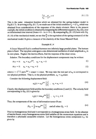
Example 8.1.4

A linear Maxwell fluid is confined between two infinitely large parallel plates. The bottom
plate is fixed. The top plate undergoes a one-dimensional oscillation of small amplitude u 0 in
its own plane. Neglect the inertia effects, find the response of the shear stress.
Solution. The boundary conditions for the displacement components may be written:

where i = ^~—\ and e = cosfttf + / s'mcat. We may take the real part of u x to correspond to
our physical problem. That is, in the physical problem, u x = u 0cosfot.
Consider the following displacement field:

Clearly, this displacement field satisfies the boundary conditions (i) and (ii). The velocity field
corresponding to Eq. (iii) is given by:

Thus, the components of the rate of deformation tensor D are:

This is a homogeneous field and it corresponds to a homogeneous stress field. In the absence
of inertia forces, every homogeneous stress field satisfies all the momentum equations and is
therefore a physically acceptable solution. Let the homogeneous stress component tr 12 be
given by