Page 126 - Introduction to Information Optics

2.6. Algorithms for Processing i 1 1

synthesis also provides us the flexibility of weighting each g n when we are
forming the SDF filter. The procedure is that we first form a correlation matrix
for all the reference functions {</„}, such as

R gQg^ (2.93)
By using the Gram-Schmidt expansion for the orthonormal set {</>,.}, we then
have

(2.94)

</>„(*) -

where the k n are normalization constants that are functions of the R tj and
where the c nj are linear combinations of the R {j with known weighting
coefficients. This tells us that when the orthonormal set is determined, the
coefficient b nj can be calculated.
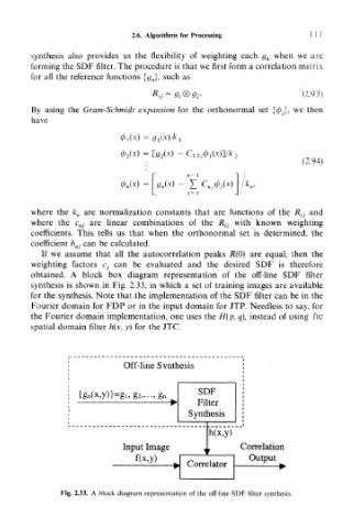
If we assume that all the autocorrelation peaks R(Q) are equal, then the
weighting factors Cj can be evaluated and the desired SDF is therefore
obtained. A block box diagram representation of the off-line SDF filter
synthesis is shown in Fig. 2.33, in which a set of training images are available
for the synthesis. Note that the implementation of the SDF filter can be in the
Fourier domain for FDP or in the input domain for JTP. Needless to say, for
the Fourier domain implementation, one uses the H(p, q), instead of using the
spatial domain filter h(x, y] for the JTC.

Off-line Synthesis

{gn(x,y)}=gl,g2,-..,gn

Input Image
f(x,y)

Fig. 2.33. A block diagram representation of the off-line SDF filter synthesis.