Page 163 - Introduction to Information Optics

148 2. Signal Processing with Optics

6. W. H. Lee, Sampled Fourier Transform Hologram Generated by Computer, Appl. Opt. 9, 639
(1970).
7. S. Yin el al, Design of a Bipolar Composite Filter Using Simulated Annealing Algorithm. Opt.
Lett., 20, 1409(1996).
8. F. T. S. Yu, White-Light Optical Processing, Wiley-Interscience, New York, (1985).
9. P. Yeh, Introduction to Photorefractive. Nonlinear Optics, Wiley, New York, (1993).
10. A. Yariv and P. Yeh, Optical Waves in Crystal, Wiley, New York, (1984).
11. J. J. Hopfield, Neural Network and Physical System with Emergent Collective Computational
Abilities, in Proc. Natl. Acad. Sci., 79, 2554 (1982).
12. D. Psaltis and N. Farhat, Optical Information Processing Based on an Associative Memory
Model of Neural Nets with Thresholding and Feedback, Opt, Lett., 10, 98 (1985).
13. F. T. S. Yu and S. Jutamulia, ed., Optical Pattern Recognition, Cambridge University Press,
Cambridge, UK, (1998).
14. F. T. S. Yu and S. Yin, Photorefractive Optics, Academic Press, Boston, (2000).

EXERCISES

2.1 Two mutually coherent beams are impinging on an observation screen.
Determine the intensity ratio by which maximum visibility can be
observed.
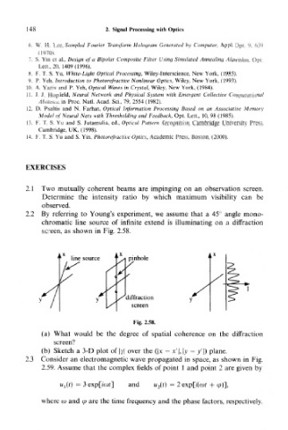
2.2 By referring to Young's experiment, we assume that a 45° angle mono-
chromatic line source of infinite extend is illuminating on a diffraction
screen, as shown in Fig. 2.58.

line source pinhole

/diffraction
screen

Fig. 2.58.
(a) What would be the degree of spatial coherence on the diffraction
screen?
(b) Sketch a 3-D plot of |y| over the (\x — x'|, |y — /|) plane.
2.3 Consider an electromagnetic wave propagated in space, as shown in Fig.
2.59. Assume that the complex fields of point 1 and point 2 are given by

u^t) = 3 exp[icof] and u z(t) — 2exp[i(a)t + <p)],

where to and (p are the time frequency and the phase factors, respectively.