Page 47 - Introduction to Information Optics

32 1. Entropy Information and Optics

then one accepts a = 0 for the received event of b. But if

p(b/ a = 0)
< 1, (1.110)
P(b/a = 1)

then one accepts a = 1.
From Eq. 1.106, we see that Eq. 1.109 implies that

P(a = 1)(C ]0 - C n ) = P(a = 0)(C 01 - C 00).

Thus, ifC 1 0 — C 11 = C 01 — C 00, then the a priori probabilities of P(a) are
equal. Note that applications of the likelihood ratio test are limited, since the
decision making takes place without knowledge of the a priori probabilities.
Thus, the results frequently are quite different from those from the minimum-
error criterion.
Although there are times when there is no satisfactory way to assign
appropriate a priori probabilities and error costs, there is a way of establishing
an optimum decision criterion; namely, the Neyman-Pearson criterion [1.9].
One allows a fixed false-alarm probability and then makes the decision in such
a way as to minimize the miss probability.

1.5.3. SIGNAL RECOVERING
An interesting problem in signal processing must be signal recovering (Le,,
restoration). The type of optimum filters is the solution based on minimization
of the mean-square error, as given by

2
2
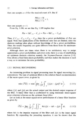
min<e (f)> = min\ lim — [L(t) -f d(tj] dt ), (1.111)
D
V^ °27'J_ 7 .
where f 0(t) and f d(t) are the actual output and the desired output response of
the filter. A linear filter that is synthesized by using minimum-mean-square
error criterion is known as the optimum linear filter.
Let us look at the mean-square-error performance of a linear filter function
as given by

T
?(0 = lim ~ { [ r HfrMt - r)dr -/,(*)T<*f, (1.112)
'-« Ll J_ r LJ^, X J J
where h(t) is the impulse response of the filter and f^t) is the input signal
function. By expanding the preceding equation, it can be shown that the