Page 101 - Introduction to Microcontrollers Architecture, Programming, and Interfacing of The Motorola 68HC12

78 Chapter 3 Addressing Modes

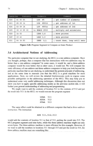
Figure 3.20. Program Segment to Compute an Inner Product

3.6 Architectural Notions of Addressing

The particular computer that we are studying, the 6812, is a one-address computer. Have
you thought, perhaps, that a computer that has instructions with two addresses may be
better than a one-address computer? In some cases, it would be, and a three-address
computer would be even better; but in other cases, it would not. We will compare the
static efficiency of one-address and three-address computers to help you look beyond the
particular machine that we are studying, to understand the general principle of addressing,
and at the same time to reassure you that the 6812 is a good machine for most
applications. Next, we will review the detailed fetch/execute cycle to expose some
possible ambiguities in the addressing operation of the 6812. This may help you to
understand some very useful addressing techniques. Although this discussion does not
show you how to apply specific addressing modes as the previous section did, it will
further your general understanding of addressing and programming.
We might want to add the contents of location 511 to the contents of 512 and put
the result into 513. In the 6812, we would execute the program segment

LDAA 511
ADDA 512
STAA 513

The same effect could be obtained in a different computer that had a three-address
instruction. The instruction

ADD 511,512,513

would add the contents of location 511 to that of 512, putting the result into 513. The
6812 program segment used nine bytes, while this three-address machine might use only
seven bytes. The three-address machine is more efficient for this example. However, if
we want to add the numbers in locations 511 through 515 and put the result in 516, the
three-address machine must use something like: