Page 94 - Introduction to Petroleum Engineering

78 PROPERTIES OF RESERVOIR ROCK
Modern numerical models often incorporate randomly chosen permeabilities in an
effort to recreate reservoir behavior. With the Dykstra–Parsons coefficient, one can com-
pare the heterogeneity of the numerical model to that of the reservoir.
To calculate the Dykstra–Parsons coefficient V , we must have a collection
DP
of permeability data for multiple layers of the same thickness in a reservoir. For
example, we can determine permeability for each 2‐ft‐thick interval in a reservoir
that is 40 ft thick so that we have a set of 20 permeabilities. Then, V can be
DP
calculated as follows:

  k  
V DP =−1exp −  ln  A   (4.23)
   k H   
where k is the arithmetic average
A
1 n
k = ∑ k i (4.24)
A
n i=1
and k is the harmonic average
H
1 = 1 ∑ 1 (4.25)
n
k H n i= 1 k i
For a reservoir with homogeneous permeability, V is 0. With increasing heteroge-
DP
neity, V increases toward 1. In most cases, V is between 0.3 and 0.9.
DP DP

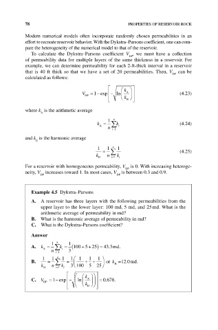
Example 4.5 Dykstra–Parsons
a. A reservoir has three layers with the following permeabilities from the
upper layer to the lower layer: 100 md, 5 md, and 25 md. What is the
arithmetic average of permeability in md?
b. What is the harmonic average of permeability in md?
C. What is the Dykstra–Parsons coefficient?

answer
1 n 1
a. k = ∑ k = (100 525 md.
++ ) = 433 .
A
n i=1 i 3
1 1 n 1 1  1 1 1 
b. = ∑ =  ++  or k = 12 0md. .

k H n i= 1 k i 3 100 5 25  H
   k  

1
C. V DP =− exp  −  ln  A  = 0 678. .


    k H   