Page 69 - Introduction to chemical reaction engineering and kinetics

3.4 Experimental Strategies for Determining Rate Parameters 51

In Figure 3.3, cA(t) plots are shown for three different values of cAO. For each value,
the initial slope is obtained in some manner, numerically or graphically, and this cor-
responds to a value of the initial rate ( --T*)~ at t = 0. Then, if the rate law is given by
equation 3.4-1,

(-rdo = ~ACL

and

ln( - rA)o = In kA + n In CA0 (3.4-7)

ByvaryingcA, in a series of experiments and measuring (- rA)O for each value of c&,,
one can determine values of kA and n, either by linear regression using equation 3.4-7,
or by nonlinear regression using equation 3.4-6.
If more than one species is involved in the rate law, as in Example 3-3, the same tech-
nique of varying initial concentrations in a series of experiments is used, and equation
3.4-7 becomes analogous to equation 3.4-4.
3.4.1.1.2 Integral methods

Test of integrated form of rate law. Traditionally, the most common method of deter-
mining values of kinetics parameters from experimental data obtained isothermally in
a constant-volume BR is by testing the integrated form of an assumed rate law. Thus,
for a reaction involving a single reactant A with a rate law given by equation 3.4-1, we
obtain, using the material balance result of equation 2.2-10,

-dCA/C; = k,dt (3.4-8)

Integration of this between the limits of cAO at t = 0, and cA at t results in
1

-&(cc’ - ciin) = kAt ( n # 1 ) (3.4-9)

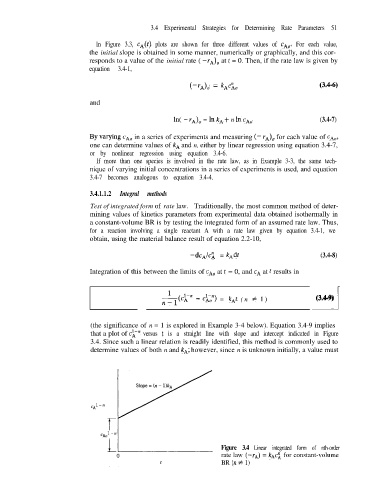
(the significance of n = 1 is explored in Example 3-4 below). Equation 3.4-9 implies
that a plot of CL” versus t is a straight line with slope and intercept indicated in Figure
3.4. Since such a linear relation is readily identified, this method is commonly used to
determine values of both n and kA; however, since n is unknown initially, a value must

Figure 3.4 Linear integrated form of nth-order
rate law (-rA) = k*cl for constant-volume
BR (n # 1)