Page 246 - MATLAB an introduction with applications

Numerical Methods ——— 231

c = diag(A,1);
end

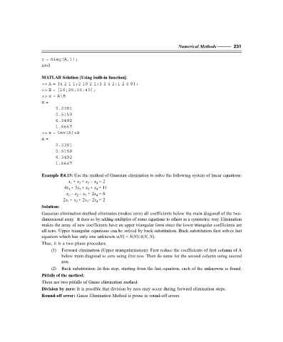
MATLAB Solution [Using built-in function]:
>> A = [4 2 1 1;2 10 2 1;1 2 4 2;1 2 4 8];
>> B = [10;20;30;40];
>> x = A\B
x =
0.2381
0.5159
6.3492
1.6667
>> x = inv(A)*B
x =
0.2381
0.5159
6.3492
1.6667

Example E4.13: Use the method of Gaussian elimination to solve the following system of linear equations:
x + x + x – x = 2
4
2
1
3
4x + 3x + x + x = 11
1
3
2
4
x – x – x + 2x = 0
2
4
3
1
2x + x + 2x – 2x = 2
4
3
2
1
Solution:
Gaussian elimination method eliminates (makes zero) all coefficients below the main diagonal of the two-
dimensional array. It does so by adding multiples of some equations to others in a symmetric way. Elimination
makes the array of new coefficients have an upper triangular form since the lower triangular coefficients are
all zero. Upper triangular equations can be solved by back substitution. Back substitution first solves last
equation which has only one unknown x(N) = b(N)/A(N, N).
Thus, it is a two phase procedure.
(1) Forward elimination (Upper triangularization): First reduce the coefficients of first column of A
below main diagonal to zero using first row. Then do same for the second column using second
row.
(2) Back substitution: In this step, starting from the last equation, each of the unknowns is found.
Pitfalls of the method:
There are two pitfalls of Gauss elimination method:
Division by zero: It is possible that division by zero may occur during forward elimination steps.
Round-off error: Gauss Elimination Method is prone to round-off errors.