Page 280 - MATLAB an introduction with applications

Optimization ——— 265

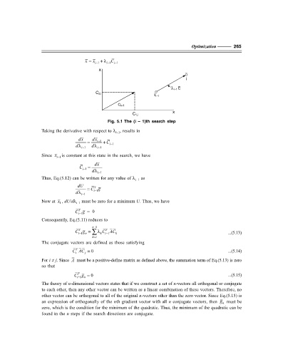
x = x i− 1 + λ i− 1 i− 1
C
x

i
λ i–1 C
C 2,i
x i–1
C i–1
x
C 1,i
Fig. 5.1 The (i – 1)th search step
Taking the derivative with respect to λ , results in
i–1
dx = dx i− 1 + C
dλ i− 1 dλ i− 1 i− 1
Since x i− 1 is constant at this state in the search, we have

dx
C i− 1 = dλ i− 1

Thus, Eq.(5.12) can be written for any value of λ as
i–1
dU = Cg
T
dλ i− 1 i− 1
Now at x , dU/dλ must be zero for a minimum U. Thus, we have
1
i–1
T
Cg = 0
i−
1
Consequently, Eq.(5.11) reduces to
n− 1
1 n ∑
T
T
Cg = λ k C AC k ...(5.13)
i−
i−
1
ki =
The conjugate vectors are defined as those satisfying
T
CAC = 0 ...(5.14)
i
j
For i ≠ j. Since A must be a positive-define matrix as defined above, the summation term of Eq.(5.13) is zero
so that
Cg = 0 ...(5.15)
T
i−
1 n
The theory of n-dimensional vectors states that if we construct a set of n-vectors all orthogonal or conjugate
to each other, then any other vector can be written as a linear combination of these vectors. Therefore, no
other vector can be orthogonal to all of the original n-vectors other than the zero vector. Since Eq.(5.15) is
an expression of orthogonally of the nth gradient vector with all n conjugate vectors, then g must be
n
zero, which is the condition for the minimum of the quadratic. Thus, the minimum of the quadratic can be
found in the n steps if the search directions are conjugate.