Page 239 - Machine Learning for Subsurface Characterization

Deep neural network architectures Chapter 7 207

2
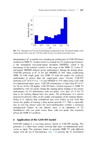
FIG. 7.9 Histogram of R for the T2 distributions synthesized for the 100 discrete depths of the
testing dataset when using the VAE-NN model having a two-dimensional latent layer.
2
determination, R , is suitable for evaluating the performance of VAE-NN-based
synthesis of NMR T2. Another metric to evaluate the T2-synthesis performance
is the normalized root-mean-square deviation (NRMSD), which is the
percentage of the residual variance to the range of the NMR T2. Lower R 2
and higher NRMSD indicate poorer performance. During the testing phase,
2
VAE-NN performs at R of 0.8 and NRMSD of 14% when synthesizing
NMR T2 with single peak. For NMR T2 with two peaks, the synthesis
performance is poorer than the single-peak cases. Overall, VAE-NN
2
performs at R of 0.75 (Fig. 7.9) and NRMSD of 15% when using VAE with
2
two-dimensional latent space. VAE-NN performance is better than R of 0.7
for 50 out of the 100 depths. VAE-NN had a limited exposure to NMR T2
distributions with two peaks during the training phase leading to the poorer
performance for T2 distributions with two peaks. Less than 1/3 of the T2
data in the training dataset have two peaks. The performance of a trained
deep neural network relies on the quality and quantity of the training dataset.
Wang et al. indicate that imbalanced data exist widely in real word that
lowers the quality of training a deep neural network [17]. This is especially
true in well log dataset when the reservoir/formation exhibits a dominant
petrophysical feature. In our dataset, there is an imbalance of T2
distributions with one peak versus those with two peaks that adversely
affects the NMR T2 synthesis.

6 Application of the GAN-NN model

GAN-NN training is a two-stage process similar to VAE-NN training. The
generator is a three-layer neural network that takes six-dimensional noise
vector as input. The generator learns to generate NMR T2 with different
shapes with the aid of discriminator. Fig. 7.10 presents the T2 distribution