Page 244 - Machine Learning for Subsurface Characterization

210 Machine learning for subsurface characterization

2
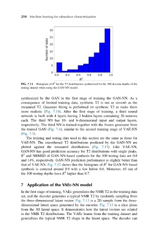
FIG. 7.12 Histogram of R for the T2 distributions synthesized for the 100 discrete depths of the
testing dataset when using the GAN-NN model.

synthesized by the GAN in the first stage of training the GAN-NN. As a
consequence of limited training data, synthetic T2 is not as smooth as the
measured T2. Gaussian fitting is performed on synthetic T2 to make them
more realistic (Fig. 7.10). After the first stage of training, a third neural
network is built with 4 layers having 2 hidden layers containing 30 neurons
each. The third NN has 10- and 6-dimensional input and output layers,
respectively. The third NN is trained together with the frozen generator from
the trained GAN (Fig. 7.4), similar to the second training stage of VAE-NN
(Fig. 7.3).
The training and testing data used in this section are the same as those for
VAE-NN. The smoothened T2 distributions predicted by the GAN-NN are
plotted against the measured distributions (Fig. 7.11). Like VAE-NN,
GAN-NN has good prediction accuracy for T2 distributions with single peaks.
2
R and NRMSD of GAN-NN-based synthesis for the 100 testing data are 0.8
and 14%, respectively. GAN-NN prediction performance is slightly better than
2
that of VAE-NN. Fig. 7.12 shows that the histogram of R for GAN-NN-based
synthesis is centered around 0.9 with a few below 0.6. Moreover, 65 out of
2
the 100 testing depths have R higher than 0.7.

7 Application of the VAEc-NN model
In the first stage of training, VAEc generalizes the NMR T2 in the training data
set, and the decoder generates a typical NMR T2 by randomly sampling from
the three-dimensional latent vector. Fig. 7.13 is a 2D sample from the three-
dimensional latent space generated by the encoder. Fig. 7.13 is a slice plane
from the 3D latent space. It demonstrates how the latent vectors are related
to the NMR T2 distributions. The VAEc learns from the training dataset and
generalizes the typical NMR T2 shape in the latent space. The decoder can