Page 31 - Machine Learning for Subsurface Characterization

16 Machine learning for subsurface characterization

2 3
measurements range from 10 ohm-m (brine-filled formation) to 10 ohm-m
(low-porosity formation) and tend to exhibit log-normal distribution. To reduce
the right skewness (i.e., mean ≫ mode) and large variance observed in the resis-
tivity data relative to other logs (features), we transformed resistivity to its log-
arithm. This reduces it skewness and variability and improves the model’s
predictive performance, as demonstrated in subsequent sections.

4.2.2 Feature scaling: Use of robust scaler
A dataset generally contains features that significantly differ from each other in
terms of magnitude, unit, and range. This tends to bias the machine learning
methods based on distance, volume, density, and gradients [16]. Without fea-
ture scaling, a few features will dominate during the model development.
For instance, the features with high magnitudes will weigh in a lot more in
the distance calculations than features with low magnitudes, which, for exam-
ple, will adversely affect k-nearest neighbor classification/regression and prin-
cipal component analysis. Without feature scaling, samples will exhibit high
density in few feature dimensions and low density in other feature dimensions.
Feature scaling is an important aspect of data preprocessing that improves the
performance of the data-driven models. For methods based on distance, volume,
and density, it is essential to ensure that the features have similar or near similar
scales for improved performance. For methods based on gradient-descent opti-
mization and other forms of gradients, it is recommended to use scaled features
for fast convergence. For neural networks, it is crucial to have the features
scaled between minimum and maximum values, preferably 0 to 1 or 1to1,
for fast and robust convergence. Notably, tree-based methods such as random
forest regression/classification, AdaBoost, and isolation forest do not require
feature scaling. Data from different logs usually range between different scales.
For example, the RHOB (1.95–2.95 g/cc), porosity (0.0–0.2 fraction) and GR
(50–250 gAPI) logs have vastly different scales.
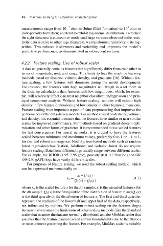
For purposes of feature scaling, we used the robust scaling method, which
can be expressed mathematically as

x i Q 1 xðÞ
x is ¼ (1.2)
Q 3 xðÞ Q 1 xðÞ
where x is is the scaled feature x for the ith sample, x i is the unscaled feature x for
the ith sample, Q 1 (x) is the first quartile of the distribution of feature x, and Q 3 (x)
is the third quartile of the distribution of feature x. The first and third quartiles
represent the medians of the lower half and upper half of the data, respectively,
not influenced by outliers. We perform robust scaling on the features (logs)
because it overcomes the limitations of other scaling methods, like the Standard
scaler that assumes the data are normally distributed and the MinMax scaler that
assumes that the feature cannot exceed certain bounds/limits due to the physics
or measurement governing the feature. For example, MinMax scaler is suitable