
Page 261 - Mathematical Models and Algorithms for Power System Optimization
P. 261
Optimization Method for Load Frequency Feed Forward Control 253
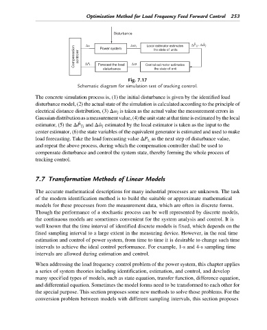
Disturbance
Compensation controler Power system Local estimator estimates
the state of units
Forecast the load
disturbance Central estimator estimates
the state of unit
Fig. 7.17
Schematic diagram for simulation test of tracking control.
The concrete simulation process is, (1) the initial disturbance is given by the identified load
disturbance model, (2) the actual state of the simulation is calculated according to the principle of
electrical distance distribution, (3) Δω j is taken as the actual value the measurement errors in
Gaussiandistributionasameasurementvalue,(4)theunitstateatthattimeisestimatedbythelocal
^
estimator, (5) the ΔP Tj and Δ^ ω j estimated by the local estimator is taken as the input to the
center estimator, (6) the state variables of the equivalent generator is estimated and used to make
load forecasting. Take the load forecasting value ΔP L as the next step of disturbance value,
and repeat the above process, during which the compensation controller shall be used to
compensate disturbance and control the system state, thereby forming the whole process of
tracking control.
7.7 Transformation Methods of Linear Models
The accurate mathematical descriptions for many industrial processes are unknown. The task
of the modern identification method is to build the suitable or approximate mathematical
models for these processes from the measurement data, which are often in discrete forms.
Though the performance of a stochastic process can be well represented by discrete models,
the continuous models are sometimes convenient for the system analysis and control. It is
well known that the time interval of identified discrete models is fixed, which depends on the
fixed sampling interval to a large extent in the measuring device. However, in the real time
estimation and control of power system, from time to time it is desirable to change such time
intervals to achieve the ideal control performance. For example, 1-s and 4-s sampling time
intervals are allowed during estimation and control.
When addressing the load frequency control problem of the power system, this chapter applies
a series of system theories including identification, estimation, and control, and develop
many specified types of models, such as state equation, transfer function, difference equation,
and differential equation. Sometimes the model forms need to be transformed to each other for
the special purpose. This section proposes some new methods to solve those problems. For the
conversion problem between models with different sampling intervals, this section proposes