Page 491 - Mathematical Techniques of Fractional Order Systems

478 Mathematical Techniques of Fractional Order Systems

We have applied the systematic search procedure (Jafari et al., 2013) into
proposed general model (16.1) in order to find chaotic cases. A simple case
has been found for
8
a 1 5 a 2 5 a 3 5 a 4 5 a 5 5 a 6 5 a 7 5 a 10 5 0
>
<
a 8 5 c ð16:9Þ
>
a 9 52 1
:
In other words, we have a new three-dimensional system
8
_ x 52 z
>
<
2
_ y 5 xz 1 asgn zðÞ ð16:10Þ
>
_ z 5 x 2 be 1 zcy 2 z
: y 2 2
in which three state variables are x, y, and z. It is noted that in system
(16.10) three positive parameters are a, b , and c ða; b; c . 0Þ.

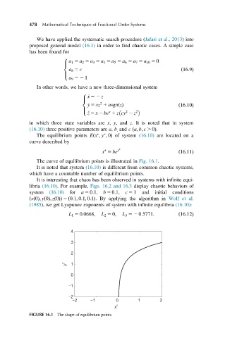
The equilibrium points Eðx ; y ; 0Þ of system (16.10) are located on a

curve described by

x 5 be y ð16:11Þ
The curve of equilibrium points is illustrated in Fig. 16.1.
It is noted that system (16.10) is different from common chaotic systems,
which have a countable number of equilibrium points.
It is interesting that chaos has been observed in systems with infinite equi-
libria (16.10). For example, Figs. 16.2 and 16.3 display chaotic behaviors of
system (16.10) for a 5 0:1, b 5 0:1, c 5 1 and initial conditions
ðxð0Þ; yð0Þ; zð0ÞÞ 5 ð0:1; 0:1; 0:1Þ. By applying the algorithm in Wolf et al.
(1985), we get Lyapunov exponents of system with infinite equilibria (16.10):
L 1 5 0:0668; L 2 5 0; L 3 52 0:5771: ð16:12Þ

4

3
2

y * 1

0
−1

−2
−2 −1 0 1 2
x *
FIGURE 16.1 The shape of equilibrium points.