Page 493 - Mathematical Techniques of Fractional Order Systems

480 Mathematical Techniques of Fractional Order Systems

1.5

1

y

0.5

0
1600 1700 1800 1900 2000
t
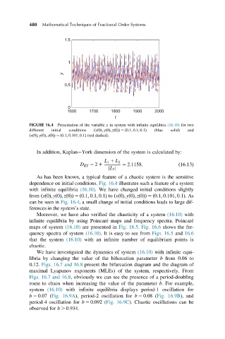
FIGURE 16.4 Presentation of the variable y in system with infinite equilibria (16.10) for two
different initial conditions ðxð0Þ; yð0Þ; zð0ÞÞ 5 ð0:1; 0:1; 0:1Þ (blue solid) and
ðxð0Þ; yð0Þ; zð0ÞÞ 5 ð0:1; 0:101; 0:1Þ (red dashed).

In addition, Kaplan York dimension of the system is calculated by:
L 1 1 L 2
D KY 5 2 1 5 2:1158: ð16:13Þ
jj
L 3
As has been known, a typical feature of a chaotic system is the sensitive
dependence on initial conditions. Fig. 16.4 illustrates such a feature of a system
with infinite equilibria (16.10). We have changed initial conditions slightly
from ðxð0Þ; yð0Þ; zð0ÞÞ 5 ð0:1; 0:1; 0:1Þ to ðxð0Þ; yð0Þ; zð0ÞÞ 5 ð0:1; 0:101; 0:1Þ.As
canbeseenin Fig. 16.4, a small change of initial conditions leads to large dif-
ferences in the system’s state.
Moreover, we have also verified the chaoticity of a system (16.10) with
infinite equilibria by using Poincare ´ maps and frequency spectra. Poincare ´
maps of system (16.10) are presented in Fig. 16.5. Fig. 16.6 shows the fre-
quency spectra of system (16.10). It is easy to see from Figs. 16.5 and 16.6
that the system (16.10) with an infinite number of equilibrium points is
chaotic.
We have investigated the dynamics of system (16.10) with infinite equi-
libria by changing the value of the bifurcation parameter b from 0.06 to
0.12. Figs. 16.7 and 16.8 present the bifurcation diagram and the diagram of
maximal Lyapunov exponents (MLEs) of the system, respectively. From
Figs. 16.7 and 16.8, obviously we can see the presence of a period-doubling
route to chaos when increasing the value of the parameter b. For example,
system (16.10) with infinite equilibria displays period-1 oscillation for
b 5 0:07 (Fig. 16.9A), period-2 oscillation for b 5 0:08 (Fig. 16.9B), and
period-4 oscillation for b 5 0:092 (Fig. 16.9C). Chaotic oscillations can be
observed for b . 0:934.