Page 498 - Mathematical Techniques of Fractional Order Systems

Dynamics, Synchronization and Fractional Order Form Chapter | 16 485

(A) (B)
1.5 0
−0.1
1
−0.2
−0.3
y 0.5 y
−0.4
−0.5
0
−0.6
−0.5 −0.7
−2 −1 0 1 2 −0.4 −0.2 0 0.2 0.4 0.6
x x
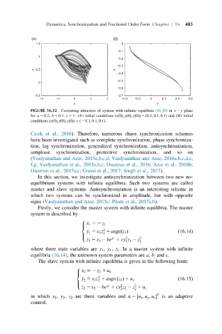
FIGURE 16.12 Coexisting attractors of system with infinite equilibria (16.10) in x 2 y plane
for a 5 0:2, b 5 0:1, c 5 1: (A) initial conditions ðxð0Þ; yð0Þ; zð0ÞÞ 5 ð0:1; 0:1; 0:1Þ and (B) initial
conditions ðxð0Þ; yð0Þ; zð0ÞÞ 5 ð2 0:1; 0:1; 0:1Þ.

Cicek et al., 2016). Therefore, numerous chaos synchronization schemes
have been investigated such as complete synchronization, phase synchroniza-
tion, lag synchronization, generalized synchronization, antisynchronization,
antiphase synchronization, protective synchronization, and so on
(Vaidyanathan and Azar, 2015a,b,c,d; Vaidyanathan and Azar, 2016a,b,c,d,e,
f,g; Vaidyanathan et al., 2015a,b,c; Ouannas et al., 2016; Azar et al., 2018b;
Ouannas et al., 2017a,c; Grassi et al., 2017; Singh et al., 2017).
In this section, we investigate antisynchronization between two new no-
equilibrium systems with infinite equilibria. Such two systems are called
master and slave systems. Antisynchronization is an interesting scheme in
which two systems can be synchronized in amplitude, but with opposite
signs (Vaidyanathan and Azar, 2015c; Pham et al., 2017a,b).
Firstly, we consider the master system with infinite equilibria. The master
system is described by

8
_ x 1 52 z 1
>
<
2
ðÞ
1
_ y 5 x 1 z 1 asgn z 1 ð16:14Þ
1
>
_ z 1 5 x 1 2 be 1 cy z 1 2 z
: y 1 2 3
1 1
where three state variables are x 1 , y 1 , z 1 . In a master system with infinite
equilibria (16.14), the unknown system parameters are a, b , and c.
The slave system with infinite equilibria is given in the following form:
8
_ x 2 52 z 2 1 u x
>
<
2
2
_ y 5 x 2 z 1 asgn ðz 2 Þ 1 u y ð16:15Þ
2
>
: 2 3
y 2
_ z 2 5 x 2 2 be 1 cy z 2 2 z 1 u z
2 2
T
in which x 2 , y 2 , z 2 are three variables and u 5 ½u x ; u y ; u z Š is an adaptive
control.