Page 540 - Mathematical Techniques of Fractional Order Systems

520 Mathematical Techniques of Fractional Order Systems

(A) (B)
0.07
0.06
0.06
0.05
0.04 0.04
0.03
MLE MLE
0.02 0.02
0.01
0 0
–0.01
–0.02 –0.02
0.395 0.4 0.405 0.41 0.415 0.42 0.425 0.6 0.605 0.61 0.615 0.62
a b
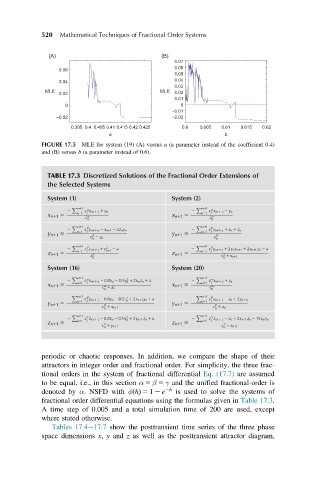
FIGURE 17.5 MLE for system (19) (A) versus a (a parameter instead of the coefficient 0.4)
and (B) versus b (a parameter instead of 0.6).

TABLE 17.3 Discretized Solutions of the Fractional Order Extensions of
the Selected Systems
System (1) System (2)
P n11 P n11
2 c α x n112j 1 y n 2 c α x n112j 2 y n
x n11 5 j51 c α j x n11 5 j51 c α j
0 0
β
P n11 P n11
β
2 c y n112j 2 x n11 2 2z n y n 2 c y n112j 1 x n 1 z n
y n11 5 j51 j β y n11 5 j51 j β
c 0 2 z n c 0
γ
γ
P n11 P n11
2
2 c z n112j 1 y n11 2 a 2 c z n112j 1 2y n y n11 1 2x n11 z n 2 a
z n11 5 j51 j γ z n11 5 j51 j γ
c 0 c 0 1 x n11
System (16) System (20)
P n11 P n11
2 c α x n112j 2 0:8x n 2 0:5y 2 1 2x n z n 1 a 2 c α x n112j 1 y n
x n11 5 j51 j n x n11 5 j51 c α j
c α 1 z n
0 0
β
β
P n11 P n11
2
2 c y n112j 2 0:8y n 2 0:5z n 1 2x n11 y n 1 a 2 c y n112j 2 x n 1 2y n z n
y n11 5 j51 j β y n11 5 j51 j β
c 0 1 x n11 c 0 1 z n
γ
γ
P n11 P n11
2
2 c z n112j 2 0:8z n 2 0:5x n 1 2y n11 z n 1 a 2 c z n112j 2 x n 2 2x n11 z n 2 15x n y n
z n11 5 j51 j γ z n11 5 j51 j γ
c 0 1 y n11 c 0 2 x n11
periodic or chaotic responses. In addition, we compare the shape of their
attractors in integer order and fractional order. For simplicity, the three frac-
tional orders in the system of fractional differential Eq. (17.7) are assumed
to be equal, i.e., in this section α 5 β 5 γ and the unified fractional-order is
denoted by α. NSFD with φðhÞ 5 1 2 e 2h is used to solve the systems of
fractional order differential equations using the formulas given in Table 17.3.
A time step of 0:005 and a total simulation time of 200 are used, except
where stated otherwise.
Tables 17.4 17.7 show the posttransient time series of the three phase
space dimensions x, y and z as well as the posttransient attractor diagram,