Page 125 - Matrix Analysis & Applied Linear Algebra

3.7 Matrix Inversion 119

Although they are not included in the simple examples of this section, you
are reminded that the pivoting and scaling strategies presented in §1.5 need to
be incorporated, and the effects of ill-conditioning discussed in §1.6 must be con-
sidered whenever matrix inverses are computed using floating-point arithmetic.
However, practical applications rarely require an inverse to be computed.
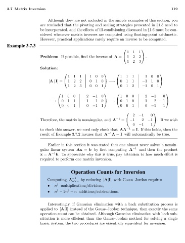
Example 3.7.3
 
111
Problem: If possible, find the inverse of A =  122  .
123
Solution:
   
111 100 111 100
[A | I]=  122 010  −→  011 −110 
123 001 012 −101

   
100 2 −10 100 2 −1 0
−→  011 −1 1 0  −→  010 −1 2 −1 
001 0 −11 001 0 −1 1

 
2 −1 0
Therefore, the matrix is nonsingular, and A −1 =  −1 2 −1  . If we wish
0 −1 1
to check this answer, we need only check that AA −1 = I. If this holds, then the
result of Example 3.7.2 insures that A −1 A = I will automatically be true.

Earlier in this section it was stated that one almost never solves a nonsin-
gular linear system Ax = b by first computing A −1 and then the product
x = A −1 b. To appreciate why this is true, pay attention to how much effort is
required to perform one matrix inversion.

Operation Counts for Inversion
−1
Computing A n×n by reducing [A|I] with Gauss–Jordan requires
3
• n multiplications/divisions,
3
2
• n − 2n + n additions/subtractions.
Interestingly, if Gaussian elimination with a back substitution process is
applied to [A|I] instead of the Gauss–Jordan technique, then exactly the same
operation count can be obtained. Although Gaussian elimination with back sub-
stitution is more efficient than the Gauss–Jordan method for solving a single
linear system, the two procedures are essentially equivalent for inversion.