Page 158 - Matrix Analysis & Applied Linear Algebra

152 Chapter 3 Matrix Algebra
4 8 12 −8 2 4 8 12 −8 2
   
 1/4 0 −6 6 1   −3/4 5 10 −10 4 
1/2 −1 −4 5 3 1/2 −1 −4 5 3
−→   −→  
−3/4 5 10 −10 4 1/4 0 −6 6 1
4 8 12 −8 2 4 8 12 −8 2
   
 −3/4 5 10 −10 4   −3/4 5 10 −10 4 
1/2 −1/5 −2 3 3 1/4 0 −6 6 1
−→   −→  
1/4 0 −6 6 1 1/2 −1/5 −2 3 3
4 8 12 −8 2
 
 −3/4 5 10 −10 4 
1/4 0 −6 6 1
−→   .
1/2 −1/51/3 1 3
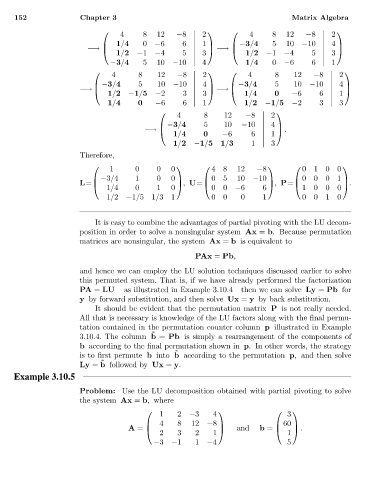
Therefore,
1 0 0 0 48 12 −8 0100
     
 −3/4 1 0 0   05 10 −10   0001 
1/4 0 1 0 00 −6 6 1000
L= , U= , P= .
1/2 −1/51/31 00 0 1 0010

It is easy to combine the advantages of partial pivoting with the LU decom-
position in order to solve a nonsingular system Ax = b. Because permutation
matrices are nonsingular, the system Ax = b is equivalent to

PAx = Pb,
and hence we can employ the LU solution techniques discussed earlier to solve
this permuted system. That is, if we have already performed the factorization
PA = LU —as illustrated in Example 3.10.4—then we can solve Ly = Pb for
y by forward substitution, and then solve Ux = y by back substitution.
It should be evident that the permutation matrix P is not really needed.
All that is necessary is knowledge of the LU factors along with the final permu-
tation contained in the permutation counter column p illustrated in Example
˜
3.10.4. The column b = Pb is simply a rearrangement of the components of
b according to the final permutation shown in p. In other words, the strategy
˜
is to first permute b into b according to the permutation p, and then solve
˜
Ly = b followed by Ux = y.
Example 3.10.5
Problem: Use the LU decomposition obtained with partial pivoting to solve
the system Ax = b, where

1 2 −3 4 3
   
 4 8 12 −8   60 
and  .
2 3 2 1 1
A =   b = 
−3 −1 1 −4 5