Page 16 - Matrix Analysis & Applied Linear Algebra

8 Chapter 1 Linear Equations

Matrix A is said to have shape or size m × n —pronounced “m by n”—
whenever A has exactly m rows and n columns. For example, the matrix
in (1.2.6) is a 3 × 4 matrix. By agreement, 1 × 1 matrices are identified with
scalars and vice versa. To emphasize that matrix A has shape m × n, subscripts
are sometimes placed on A as A m×n . Whenever m = n (i.e., when A has the
same number of rows as columns), A is called a square matrix. Otherwise, A
is said to be rectangular. Matrices consisting of a single row or a single column
are often called row vectors or column vectors, respectively.
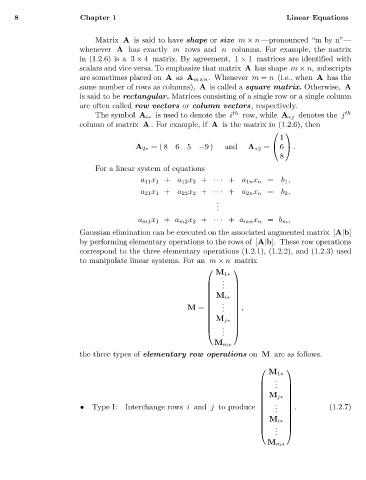
The symbol A i∗ is used to denote the i th row, while A ∗j denotes the j th
column of matrix A . For example, if A is the matrix in (1.2.6), then
 
1
A 2∗ = (865 −9 ) and A ∗2 =   .
6
8
For a linear system of equations
a 11 x 1 + a 12 x 2 + ··· + a 1n x n = b 1 ,
a 21 x 1 + a 22 x 2 + ··· + a 2n x n = b 2 ,
.
.
.
a m1 x 1 + a m2 x 2 + ··· + a mn x n = b m ,
Gaussian elimination can be executed on the associated augmented matrix [A|b]
by performing elementary operations to the rows of [A|b]. These row operations
correspond to the three elementary operations (1.2.1), (1.2.2), and (1.2.3) used
to manipulate linear systems. For an m × n matrix
 
M 1∗
.
 . . 
 
 
 M i∗ 
 . 
M =  . .  ,
 
 
 M j∗ 
.
 
.
 . 
M m∗
the three types of elementary row operations on M are as follows.
 
M 1∗
.
 . . 
 
 
 M j∗ 
 . 
• Type I: Interchange rows i and j to produce  .  . (1.2.7)
 . 
 
 M i∗ 
.
 
.
 . 
M m∗