Page 209 - Matrix Analysis & Applied Linear Algebra

204 Chapter 4 Vector Spaces
Example 4.4.7

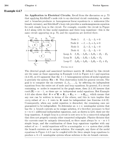
An Application to Electrical Circuits. Recall from the discussion on p. 73
that applying Kirchhoff’s node rule to an electrical circuit containing m nodes
and n branches produces m homogeneous linear equations in n unknowns (the
branch currents), and Kirchhoff’s loop rule provides a nonhomogeneous equation
for each simple loop in the circuit. For example, consider the circuit in Figure
4.4.2 along with its four nodal equations and three loop equations—this is the
same circuit appearing on p. 73, and the equations are derived there.
E 1 E 2
R 1 1 R 2 Node 1: I 1 − I 2 − I 5 =0
I 1 I 2
Node 2: − I 1 − I 3 + I 4 =0
A B
R 5
E 3 Node 3: I 3 + I 5 + I 6 =0
I 5
R 3 R 6
2 4 Node 4: I 2 − I 4 − I 6 =0
3
I 3 I 6
Loop A: I 1 R 1 − I 3 R 3 + I 5 R 5 = E 1 − E 3
C
Loop B: I 2 R 2 − I 5 R 5 + I 6 R 6 = E 2
I 4
Loop C: I 3 R 3 + I 4 R 4 − I 6 R 6 = E 3 + E 4
R 4
E 4
Figure 4.4.2
The directed graph and associated incidence matrix E defined by this circuit
are the same as those appearing in Example 4.4.6 in Figure 4.4.1 and equation
(4.4.16), so it’s apparent that the 4 × 3 homogeneous system of nodal equations
is precisely the system Ex = 0. This observation holds for general circuits. The
goal is to compute the six currents I 1 ,I 2 ,...,I 6 by selecting six independent
equations from the entire set of node and loop equations. In general, if a circuit
containing m nodes is connected in the graph sense, then (4.4.18) insures that
rank (E)= m − 1, so there are m independent nodal equations. But Example
T
4.4.6 also shows that 0 = e E = E 1∗ + E 2∗ + ··· + E m∗ , which means that
any row can be written in terms of the others, and this in turn implies that
every subset of m − 1rows in E must be independent (see Exercise 4.4.13).
Consequently, when any nodal equation is discarded, the remaining ones are
guaranteed to be independent. To determine an n × n nonsingular system that
has the n branch currents as its unique solution, it’s therefore necessary to find
n−m+1 additional independent equations, and, as shown in §2.6, these are the
loop equations. A simple loop in a circuit is now seen to be a connected subgraph
that does not properly contain other connected subgraphs. Physics dictates that
the currents must be uniquely determined, so there must always be n − m +1
simple loops, and the combination of these loop equations together with any
subset of m − 1 nodal equations will be a nonsingular n × n system that yields
the branch currents as its unique solution. For example, any three of the nodal
equations in Figure 4.4.2 can be coupled with the three simple loop equations to
produce a 6 × 6 nonsingular system whose solution is the six branch currents.